A historical overview of atmosphere and ocean dynamics
Atmosphere and Ocean Dynamics, Lecture 1: notes
How the large-scale motions of the atmosphere and the ocean came to be understood, and computed, in the order of the dates, from Torricelli’s barometer (1643) to the first ocean and climate models (1969). These notes discuss the weight of the air and the gas law; Hadley’s argument, angular momentum, the Coriolis force and the geostrophic wind; the tides of Newton and Laplace; the equations of Euler, Navier and Stokes; circulation and vorticity; forecasting as an initial-value problem, from Bjerknes and Richardson to the first computer forecast, in 1950; Rossby waves and blocking; and the wind-driven ocean, from Ekman to Stommel and Munk.
1 Atmosphere and ocean dynamics
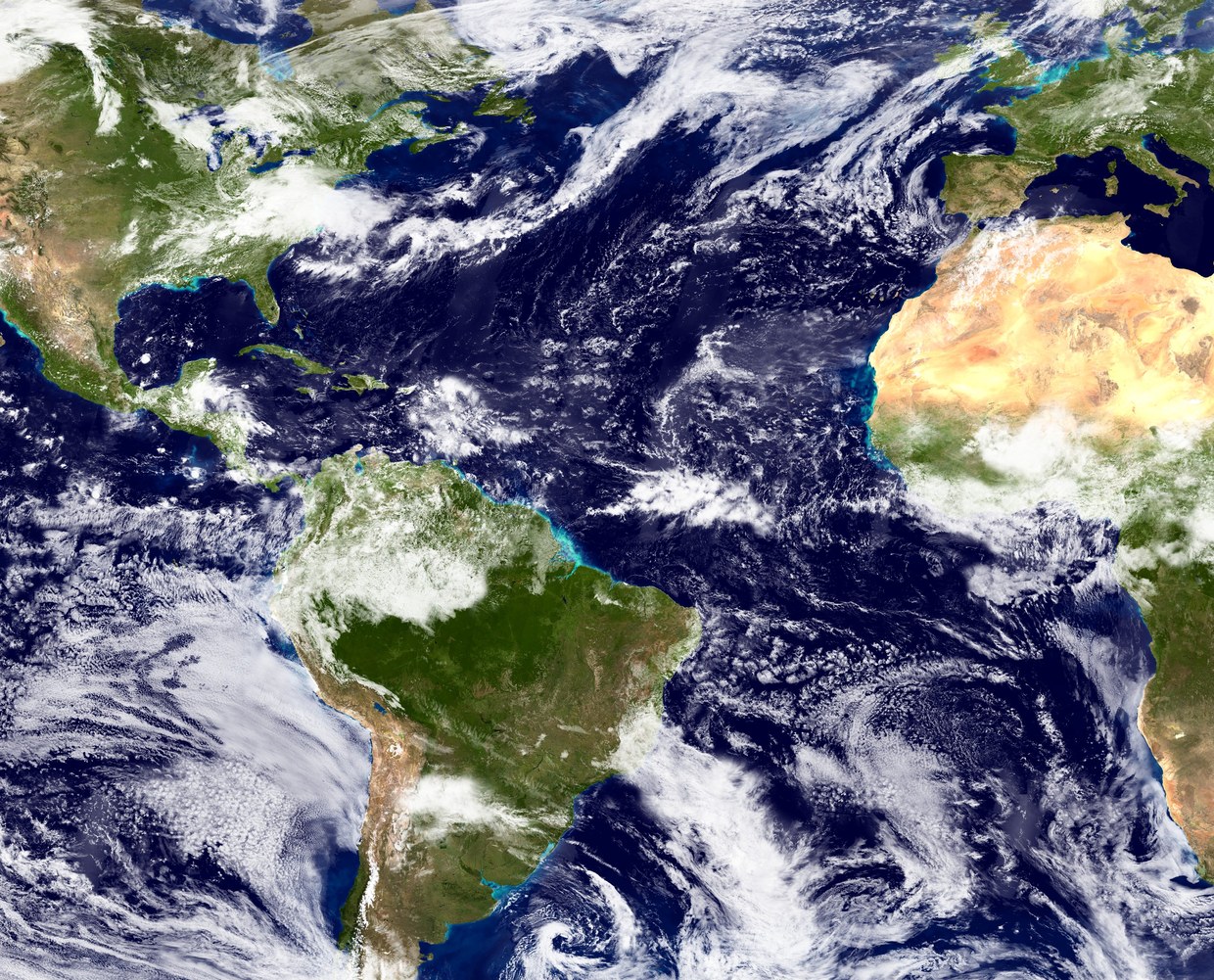
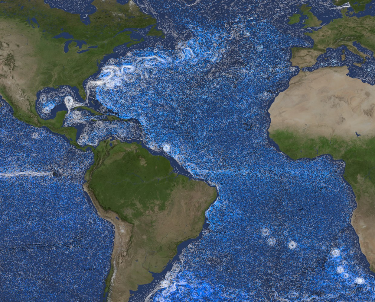
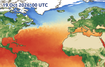
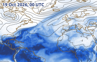
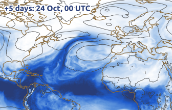
The maps of Figure 1 show the same part of the Atlantic at the same scale: cyclones and fronts about 1000 km across, travelling eastward in middle latitudes; and the clockwise North Atlantic gyre, whose return flow is crowded into a narrow, fast current on its western side, the Gulf Stream. Averaged around latitude circles, the surface winds blow westward in the tropics (the trade winds) and eastward in middle latitudes, and every subtropical gyre has a fast western current (Gulf Stream, Kuroshio, Brazil, Agulhas) (Vallis 2017, Ch. 14 and 19). Both fluids are thin layers on a sphere of radius \(a \approx 6371\) km turning at \(\Omega \approx 7.29\times10^{-5}\,\mathrm{s^{-1}}\), driven by uneven heating.

2 Scales of motion
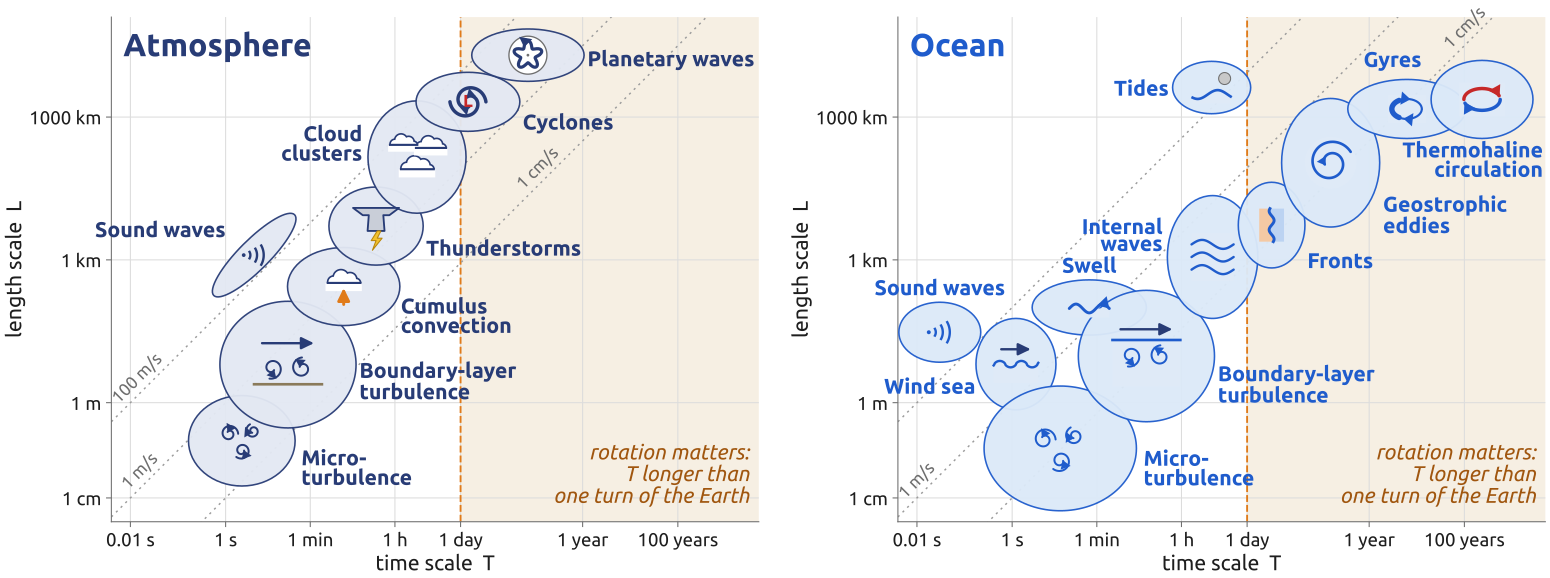
Figure 2 ranks the motions of the air and of the sea by their typical length \(L\) and time \(T\), on logarithmic axes from centimetres and seconds to the size of the Earth and centuries (Cushman-Roisin and Beckers 2011, fig. 1.7, after a diagram by H. von Storch). In both fluids the ellipses climb along a diagonal: large motions are slow ones. Their speed \(U = L/T\) is constant along lines of slope one: weather systems move at about 10 m/s, ocean eddies and gyres at about 1 cm/s. The ocean is slower and its eddies are smaller than their atmospheric counterparts (Cushman-Roisin and Beckers 2011, sec. 1.7 and Table 1.2, which also gives the velocity scales).
When does the rotation of the Earth matter? A motion feels it when it lasts about one turn of the Earth or longer, \(T \gtrsim 2\pi/\Omega \approx 1\) day, with \(\Omega \approx 7.29\times10^{-5}\,\mathrm{s^{-1}}\) the rotation rate; a faster motion feels it too if a parcel takes about a day or longer to cross it, \(2\pi U/(\Omega L) \lesssim 1\) (Cushman-Roisin and Beckers 2011, sec. 1.5, eqs. 1.2–1.3). The shaded part of Figure 2 is the first criterion: cyclones, planetary waves, tides, ocean eddies and gyres, the large-scale motions of the opening maps. Sound waves, turbulence and convection are too small and too fast to feel the rotation.
3 On the shoulders of giants
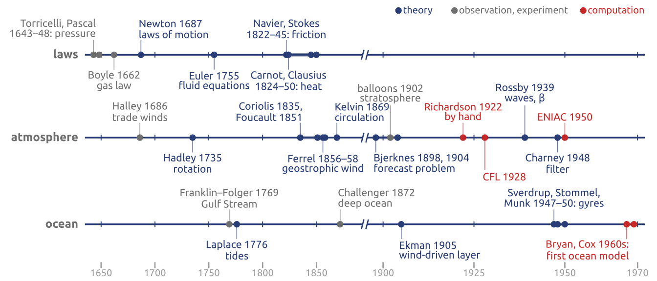
Newton wrote the line of the slide to Robert Hooke (5 February 1675/6), in a letter on optics; there the giants are Descartes and Hooke (Newton 1676). The image goes back to Bernard of Chartres, in the twelfth century: dwarfs on the shoulders of giants see farther because the giants lift them up (Merton 1965). The sections below follow the dates of the giants’ main contributions; overviews of the whole story are Vallis (2016) and Lorenz (1983).
4 Torricelli, Pascal (1643–48): the weight of the air
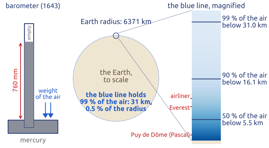
In 1643 Evangelista Torricelli turned a tube full of mercury upside down into a dish of mercury: the column fell to about 760 mm, held up by the weight of the air on the dish. On 19 September 1648, at Blaise Pascal’s request, Florin Périer carried the barometer up the Puy de Dôme, about 1000 m above Clermont-Ferrand, and found the column about 85 mm lower: less air above (Pascal 1648). Pressure \(p\) is the weight of the air above a unit area; with \(\rho\) the density, \(z\) the height and \(g \approx 9.81\ \mathrm{m\,s^{-2}}\), \[ \frac{\partial p}{\partial z} = -\rho g , \] the hydrostatic balance (Vallis 2017, sec. 1.3.3). A square metre carries \(p_0/g \approx 10\) tonnes of air (\(p_0 \approx 1013\) hPa at sea level); the fraction of the air below \(z\) is \(1 - p(z)/p_0\), half below 5.5 km and 99 % below 31 km (Figure 3).
5 Boyle (1662): the spring of the air
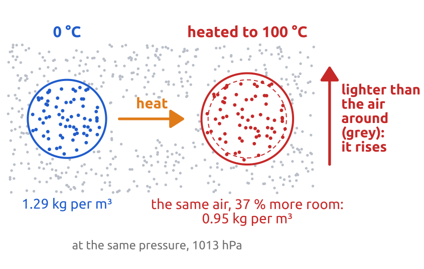
Robert Boyle reported in 1662 that, at a fixed temperature, pressure times volume stays the same. That heated air expands was known only qualitatively: Halley (1686) calls it “rarified, and less ponderous” (Halley 1686, 165). Jacques Charles (1787) and Joseph Louis Gay-Lussac (1802) found that, at a fixed pressure, all gases expand by the same fraction for the same warming: the volume grows linearly with temperature, in proportion to what was later called the absolute temperature \(T\). Together the two laws give the ideal gas law \[ p = \rho R T , \] with \(T\) in kelvin and \(R = 287\ \mathrm{J\,kg^{-1}\,K^{-1}}\) for dry air (Vallis 2017, sec. 1.4). Heated from \(0\) to \(100\,^\circ\)C at constant pressure, the volume of air grows by the factor \(373/273 = 1.37\) and its density falls from 1.29 to \(0.95\ \mathrm{kg\,m^{-3}}\) (Figure 4): the denser air around pushes it up.
6 Halley (1686): the Sun drives the winds
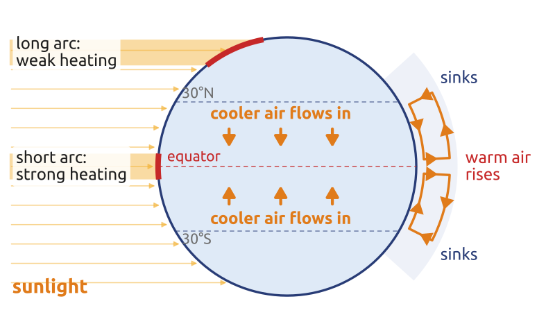
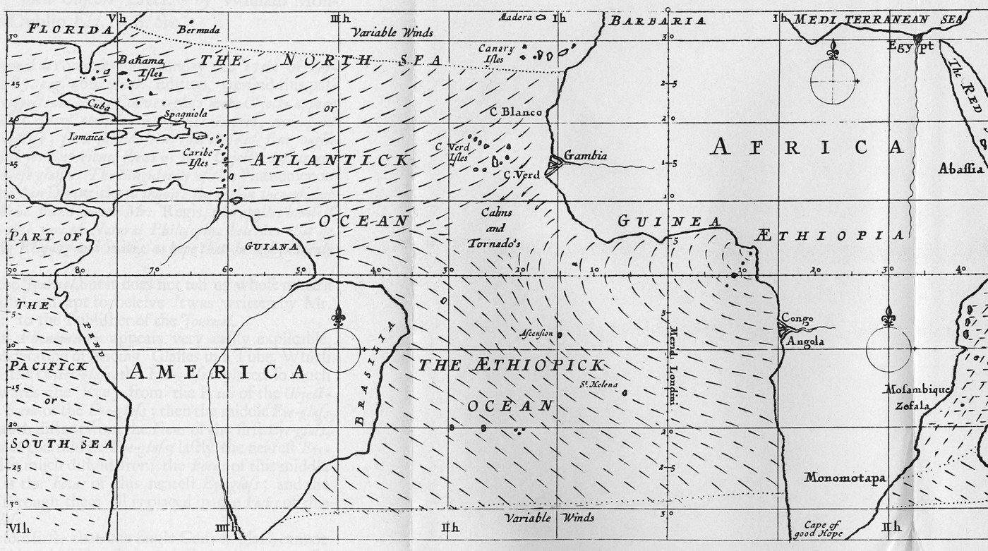
Edmond Halley mapped the trade winds from sailors’ reports (Figure 6) and explained them by heating (Halley 1686, 165–67): the same beam of sunlight heats a small area near the equator and a large one near the poles (Figure 5; at the equinoxes the daily mean heating per unit area goes as \(\cos\varphi\), \(\varphi\) being the latitude). Heated air rises, and cooler air flows in at the surface from both sides. Heating gives no east–west direction, though, and his reason for the westward turn, that the heating follows the Sun’s daily westward motion, is wrong (Lorenz 1983, 731). What lasts is the driver: the tropics gain heat, the poles lose it, and winds and currents carry it poleward. (He is also the Halley of the comet, whose return in 1758 he predicted.)

7 Newton (1687): motion and gravity
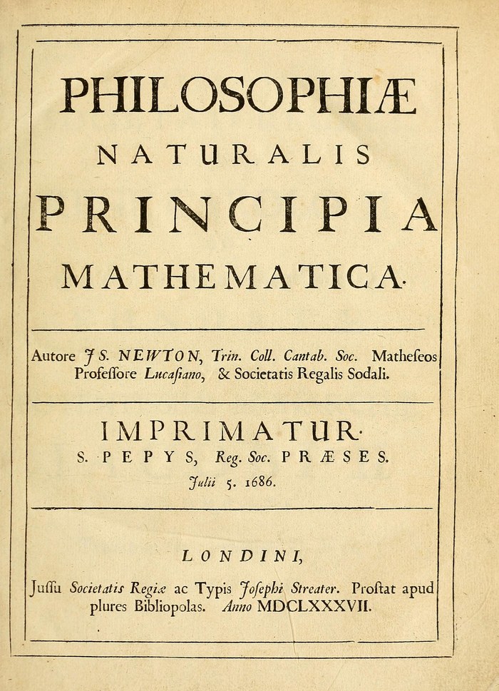
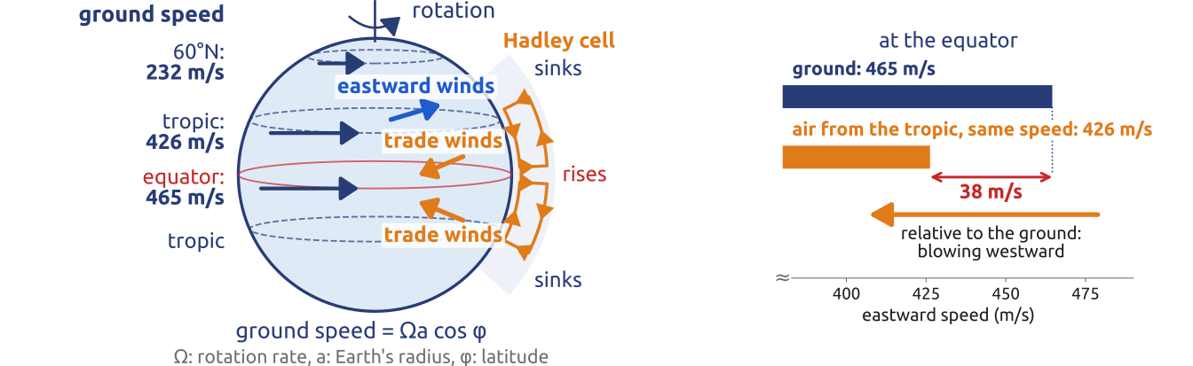
The Principia (Newton 1687) (Figure 7) set out the laws of motion and universal gravitation. Inertia holds in a frame that does not rotate (the fixed stars), not on the turning ground. The second law, \(\mathbf{F} = m\,\mathbf{a}\), is what Euler later wrote for every parcel of fluid. Gravitation, \(F = G m_1 m_2/r^2\) between masses \(m_1\), \(m_2\) at a distance \(r\) (\(G \approx 6.67\times10^{-11}\ \mathrm{N\,m^2\,kg^{-2}}\)), gives the weight of the air and the tides. Halley persuaded Newton to write the book and paid for its printing. Newton’s laws hold the answer to Halley’s question: with no east–west force, air moving towards the equator does not take up the faster eastward motion of the ground under it, and lags behind; by how much is settled by angular momentum (Section 9).

8 Hadley (1735): rotation turns the winds
George Hadley (1735) found the cause in the Earth’s rotation (Figure 8). The ground moves east at \(\Omega a\cos\varphi\): 465 m/s at the equator, 426 m/s at the Tropic of Cancer (\(23.4^\circ\)N). Air from the tropic reaching the equator, “having a less Velocity than the Parts of the Earth it arrives at” (p. 60), lags behind the ground: a westward wind, which with the motion towards the equator gives the trade winds, towards the southwest in the northern hemisphere and the northwest in the southern; air returning poleward aloft runs ahead of the ground. The lag, 38 m/s, exceeds “the greatest Storm” (p. 61), while trade winds blow at 5–10 m/s; Hadley invoked friction with the surface (Persson 2006, 33–34). These notes name winds by where they go (eastward, westward), as the eastward velocity \(u\) does; meteorologists usually name them by where they come from: a “westerly” (Italian vento da ovest) blows from the west, that is, eastward.
9 Angular momentum
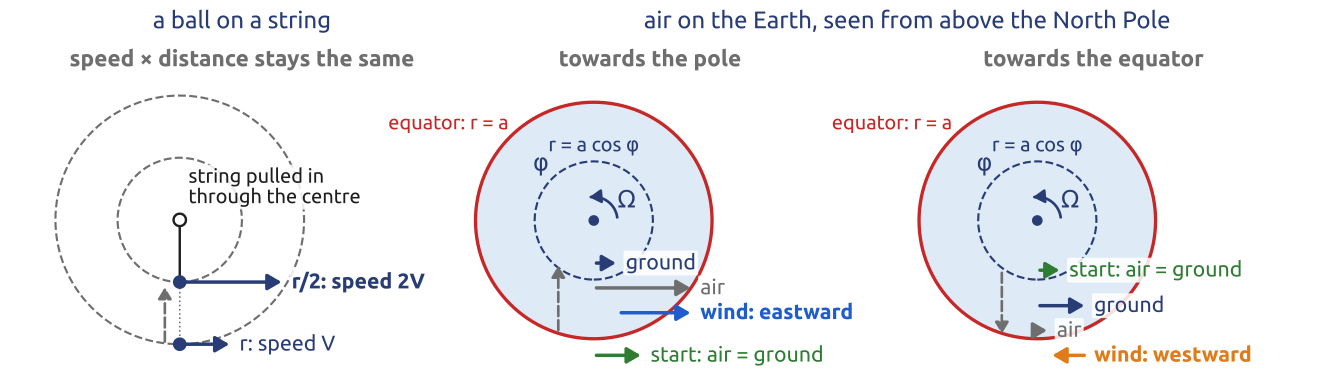
Per unit mass, the angular momentum about an axis is \(m = r\,v\), with \(r\) the distance to the axis and \(V\) the speed around it; a force towards the axis cannot change it (Figure 9, left). On the Earth, \(r = a\cos\varphi\) and the eastward speed in space is \(V = \Omega a\cos\varphi + u\), with \(u\) the eastward wind relative to the ground (\(u < 0\): westward), so \[ m = (\Omega a\cos\varphi + u)\,a\cos\varphi \] (Vallis 2017, sec. 14.2). Without an east–west force (friction, an east–west pressure difference), \[ \frac{Dm}{Dt} = \frac{\partial m}{\partial t} + \mathbf{u}\cdot\nabla m = 0 , \] with \(\mathbf{u}\) the velocity and \(D/Dt\) the material derivative, the change following the air. For a ring of air at rest relative to the ground at latitude \(\varphi_0\) that moves to \(\varphi\), the same \(m\) at both latitudes, \[ \underbrace{\Omega a\cos\varphi_0\;a\cos\varphi_0}_{m\text{ at }\varphi_0} = \underbrace{(\Omega a\cos\varphi + u)\,a\cos\varphi}_{m\text{ at }\varphi}, \] gives its wind at \(\varphi\), \[ u = \Omega a\left(\frac{\cos^2\varphi_0}{\cos\varphi} - \cos\varphi\right): \] eastward (\(u > 0\)) for poleward motion, it runs ahead of the ground; westward for equatorward motion, it lags behind. Hadley kept the eastward speed in space instead, \(\Omega a\cos\varphi_0 = \Omega a\cos\varphi + u\), so \(u = \Omega a\,(\cos\varphi_0 - \cos\varphi)\), which no law conserves: right directions, about half the deflection (Persson 2006, 32). Both are far stronger than observed: \(m\) is nearly kept only aloft (the subtropical jet); friction slows the trade winds, and eddies (the weather systems) maintain the mid-latitude surface winds (Lorenz 1983).
10 In class: Hadley and angular momentum
Exercise 1 — Hadley’s argument and angular momentum. Air at rest over the equator rises and moves towards the pole, high up. What is its wind \(u\) at latitude \(\varphi\) if it keeps (a) its eastward speed in space \(V\), as Hadley (1735) assumed? (b) its angular momentum \(m\)? Compute \(u\) at \(10^\circ\), \(20^\circ\) and \(30^\circ\) and compare with the observed subtropical jet, 30–40 m/s. What could slow the air down?
| \(u\) (m/s) | \(10^\circ\) | \(20^\circ\) | \(30^\circ\) |
|---|---|---|---|
| (a) keeping its speed in space (Hadley) | |||
| (b) keeping its angular momentum | |||
| observed (subtropical jet) | 30–40 |
Constants: \(\Omega = 7.29\times10^{-5}\,\mathrm{s^{-1}}\), \(a = 6371\) km.
(c) To hand in: the other way round. Air at rest at \(30^\circ\) moves towards the equator, near the ground. Compute \(u\) at \(20^\circ\), \(10^\circ\) and \(0^\circ\) with (a) and (b), and compare with the trade winds, blowing westward at 5–10 m/s. What slows the air down here?
11 Newton’s tide and the real ocean
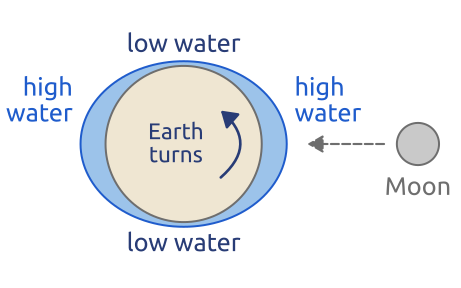
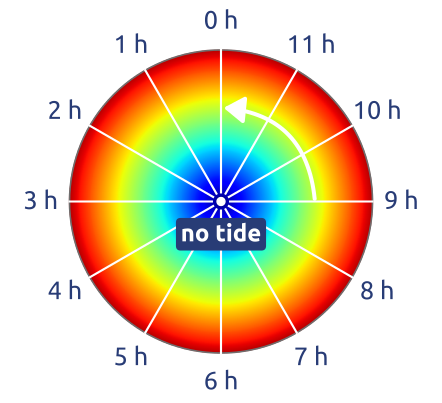
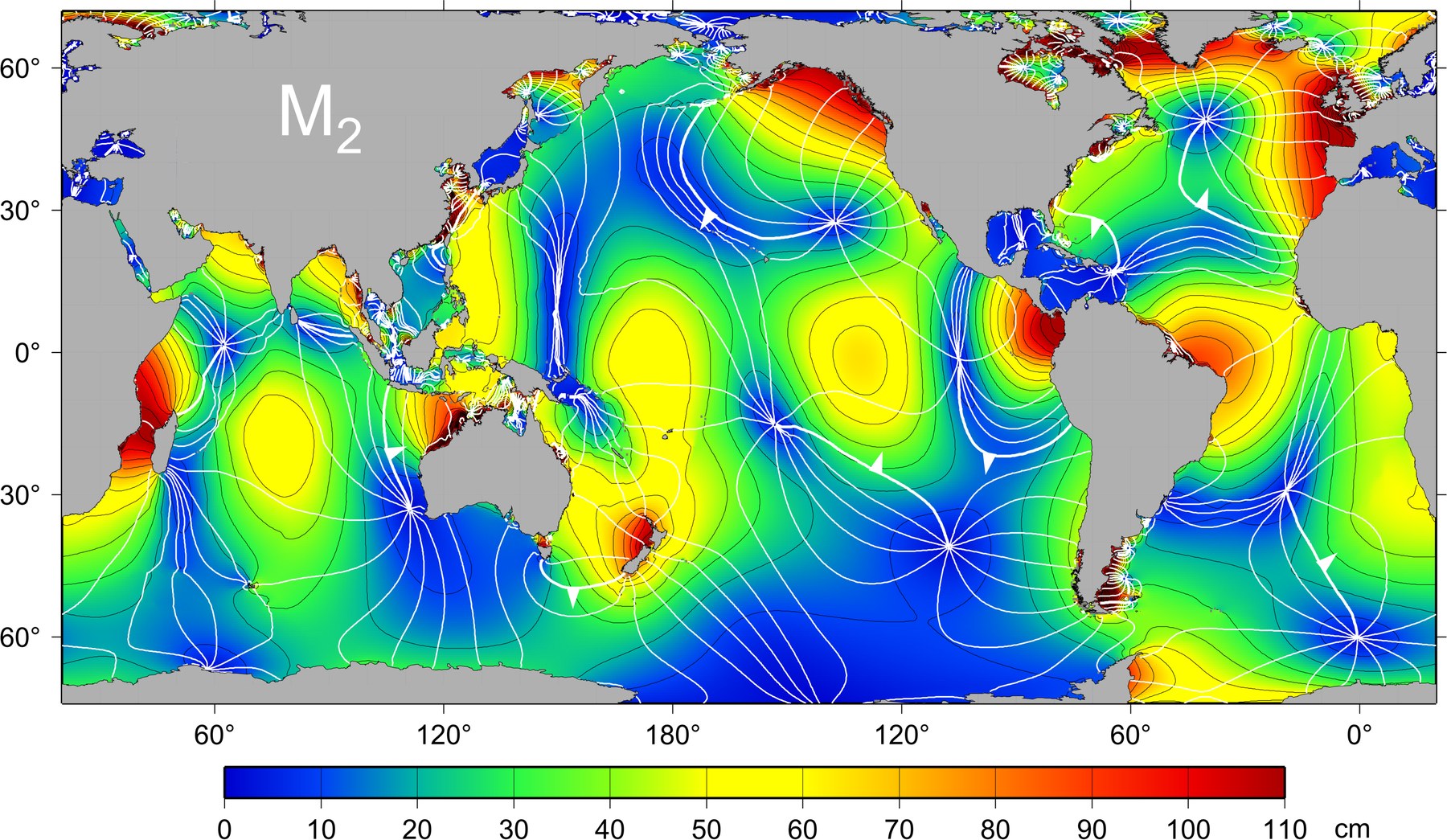
Newton explained the tide-raising force: the difference between the Moon’s (or the Sun’s) pull at a point of the Earth and at its centre (Hendershott 1981, 293). An ocean taking at each moment the shape this force asks for, the equilibrium tide of Daniel Bernoulli (1738) (Hendershott 1981, 318), has two bulges, under the Moon and opposite (Figure 10 (a)); its main term, the lunar semidiurnal tide M2 (period 12.42 h), is about 24 cm at the equator, falling as \(\cos^2\varphi\) (Hendershott 1981, 294). The real tide differs: high water comes hours after the Moon’s passage, with a delay that varies from port to port; open-ocean amplitudes reach 1 m, coastal ranges over 15 m (Bay of Fundy); and at amphidromic points the sea neither rises nor falls; the first one recorded was probably in the North Sea, from Captain Hewett’s soundings of 1840 (Hendershott 1981, 318, quoting Darwin, who writes “Hewitt”). On a map of one constituent (Figure 11), cotidal lines join places with high water at the same time; the crest turns around each amphidromic point (Figure 10 (b)), in a rotating basin anticlockwise in the northern hemisphere (Hendershott 1981, 299), as most observed amphidromes do.
12 Euler (1755): the equations of a fluid
Leonhard Euler (memoir read in Berlin in 1755, printed in 1757 (Euler 1757)) treated the fluid as a continuum, with velocity \(\mathbf{u}\), pressure \(p\) and density \(\rho\) at every point, and wrote Newton’s second law for every parcel: \[ \frac{D\mathbf{u}}{Dt} = -\frac{1}{\rho}\nabla p - \nabla\Phi , \qquad \frac{\partial\rho}{\partial t} + \nabla\cdot(\rho\mathbf{u}) = 0 , \] with \(D/Dt = \partial/\partial t + \mathbf{u}\cdot\nabla\) the rate of change following the parcel and \(\Phi\) the geopotential (\(\Phi = gz\) near the ground) (Vallis 2017, secs. 1.1–1.3). The second, the continuity equation, keeps mass. Euler’s fluid has no friction: d’Alembert had shown in 1752 that a body moving steadily through it feels no drag. The name Euler’s equations is that of the frictionless system (Chorin and Marsden 1993, sec. 1.1); with friction it is the Navier–Stokes equation (Vallis 2017, sec. 1.3.2).
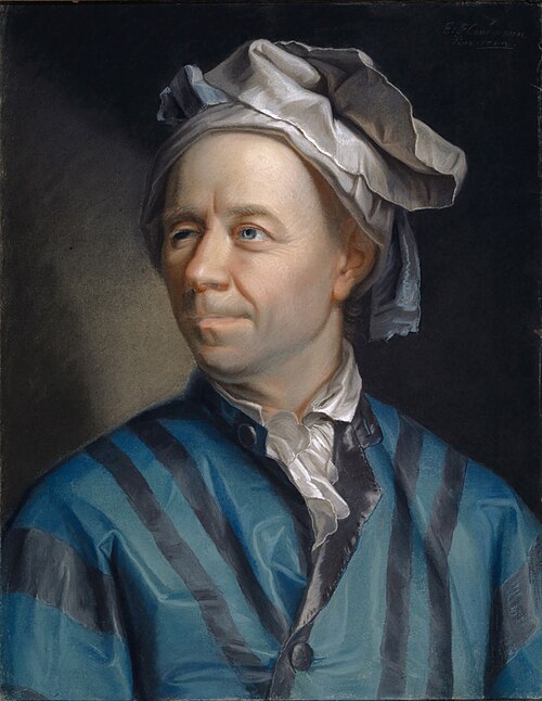

13 Laplace (1776): the tides of a rotating ocean
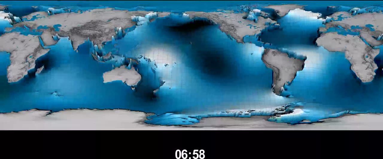
Pierre-Simon Laplace (1775–76) treated the ocean as a fluid with inertia on the rotating Earth (Hendershott 1981, 292, 295, 318). With \(\eta\) the sea-surface height, \(\mathbf{u}\) the horizontal current, \(H\) the depth, \(\mathbf{k}\) the local vertical, \(f = 2\Omega\sin\varphi\) the Coriolis parameter (Section 17) and the equilibrium tide \(\eta_{eq}\) as forcing, his tidal equations are, in a local flat form (he wrote them on the sphere), \[ \begin{aligned} \frac{\partial \mathbf{u}}{\partial t} + f\,\mathbf{k}\times\mathbf{u} &= -g\nabla(\eta - \eta_{eq}),\\ \frac{\partial \eta}{\partial t} + \nabla\cdot(H\mathbf{u}) &= 0 : \end{aligned} \] the linear shallow water equations, with the rotation term sixty years before Coriolis. The ocean cannot follow the Moon: the point under it moves round the equator at about 450 m/s, long waves in 4 km of water at \(\sqrt{gH} \approx 200\) m/s. The tide becomes waves lagging the forcing, blocked by the continents, turned by the rotation, amplified by resonance in some basins. Kelvin’s harmonic method (about 1870), still used for tide tables, takes the frequencies from astronomy and each amplitude and phase from tide gauges (Hendershott 1981, 318); today the tide is measured from satellites and computed from Laplace’s equations (Figure 13).
14 Navier (1822), Stokes (1845): friction
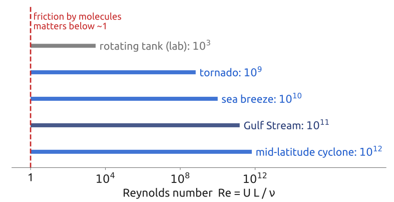
Claude-Louis Navier (read 1822, printed 1827 (Navier 1827)) and George Gabriel Stokes (Stokes 1845) added the friction between layers of fluid: at constant density the momentum equation gains \(\nu\nabla^2\mathbf{u}\), with \(\nabla^2\) the Laplacian and \(\nu\) the kinematic viscosity (\(1.5\times10^{-5}\ \mathrm{m^2\,s^{-1}}\) for air, \(10^{-6}\) for water): the Navier–Stokes equations. For a flow of speed \(U\) and size \(L\), acceleration (\(U^2/L\)) over friction (\(\nu U/L^2\)) is the Reynolds number \(Re = UL/\nu\) (Reynolds 1883; Cushman-Roisin and Beckers 2011, sec. 4.5): about \(7\times10^{11}\) for a cyclone (\(U = 10\) m/s, \(L = 1000\) km; Figure 14). Molecular friction is negligible, but the flow is turbulent, and eddies down to millimetres mix momentum and heat. Resolving them would take about \(5\times10^{27}\) grid points (\(5\times10^{18}\ \mathrm{m^3}\) of air on a 1 mm grid): models compute the large scales and parameterize the rest.
15 Carnot (1824), Clausius (1850): heat and work
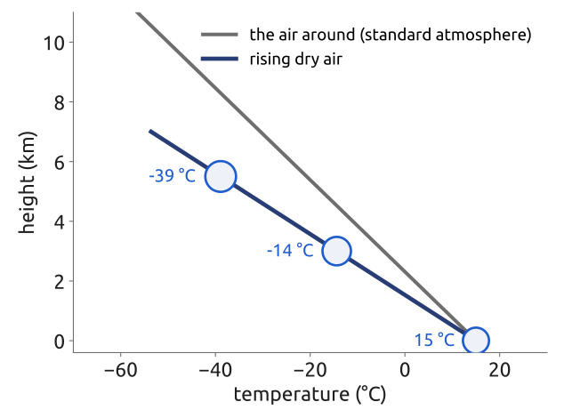
Sadi Carnot (1824) studied heat engines, the start of the second law of thermodynamics; Rudolf Clausius (1850) related heat and work and stated the first law, the conservation of energy (Clausius 1850; Wallace and Hobbs 2006, ch. 3). For air with specific heat \(c_p = 1004\ \mathrm{J\,kg^{-1}\,K^{-1}}\) heated at the rate \(Q\) per unit mass, \[ c_p\frac{DT}{Dt} - \frac{1}{\rho}\frac{Dp}{Dt} = Q . \] Rising air meets lower pressure, expands and cools: with \(Q = 0\) and \(Dp/Dt = -\rho g w\) (hydrostatic pressure, rising speed \(w\)), \(c_p\,DT/Dt = -g w\), a cooling of \(g/c_p \approx 9.8\) K per km (Figure 15). Hence cold mountain tops, and clouds in rising air, where condensing vapour releases latent heat; the observed mean decrease is about 6.5 K/km. A parcel pushed up and colder than its new surroundings sinks back: the atmosphere is usually stably stratified.
16 Coriolis (1835): a planar rotating frame (disk)
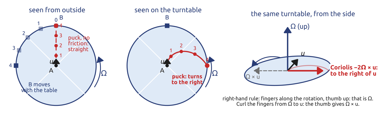
On the turning Earth, Newton’s laws gain two apparent forces (Vallis 2017, sec. 2.1). The centrifugal force, independent of the motion, is absorbed into gravity and the geopotential \(\Phi\) (exactly; the approximation comes after, when the surfaces of constant \(\Phi\) are taken as spheres). The Coriolis force, \(-2\boldsymbol{\Omega}\times\mathbf{u}\) per unit mass, acts on the velocity \(\mathbf{u}\) relative to the Earth; \(\boldsymbol{\Omega}\) is the rotation vector, along the axis towards the North Star (right-hand rule), of size \(2\pi/(\text{sidereal day}) \approx 7.29\times10^{-5}\,\mathrm{s^{-1}}\): \[ \frac{D\mathbf{u}}{Dt} + 2\boldsymbol{\Omega}\times\mathbf{u} = -\frac{1}{\rho}\nabla p - \nabla\Phi . \] Perpendicular to \(\mathbf{u}\), the force turns the motion and does no work (Figure 16). Gaspard-Gustave Coriolis derived it in 1835 for machines such as water wheels (Coriolis 1835; Persson 1998, 1377–78); the terms were already in Laplace’s tidal equations (Hendershott 1981, 295; Vallis 2016, 5). Meteorology learned the deflection through Foucault and Ferrel, and the name “Coriolis force” spread there only in the twentieth century (Persson 1998, 1383).
17 Foucault (1851): the local rotation
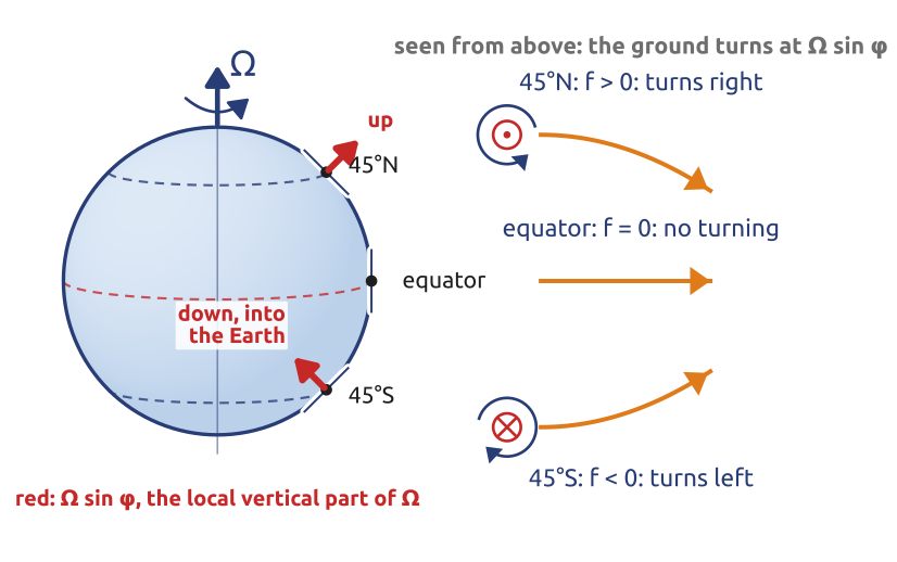
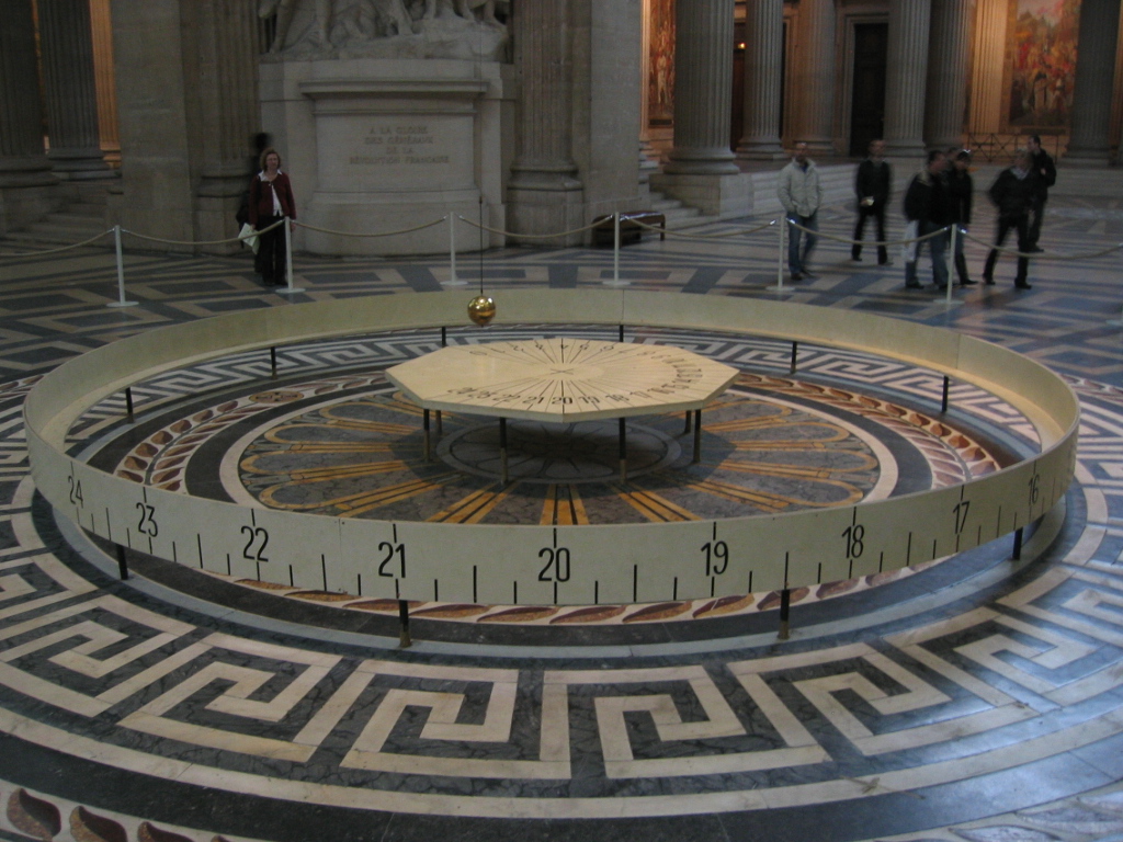
At latitude \(\varphi\), \(\boldsymbol{\Omega}\) has a part \(\Omega\sin\varphi\) along the local vertical \(\mathbf{k}\) (up in the northern hemisphere, down in the southern) and a part \(\Omega\cos\varphi\) along the local north (Figure 17). Only the vertical part turns horizontal motion: \[ -2\Omega\sin\varphi\;\mathbf{k}\times\mathbf{u} = -f\,\mathbf{k}\times\mathbf{u}, \qquad f = 2\Omega\sin\varphi , \] the Coriolis parameter. As \(\mathbf{k}\times\mathbf{u}\) is \(\mathbf{u}\) turned \(90^\circ\) to the left, the force points right of the motion in the northern hemisphere (\(f > 0\)), left in the southern, and vanishes at the equator; the \(\Omega\cos\varphi\) part is neglected for thin layers. At Milan (\(f \approx 1.04\times10^{-4}\,\mathrm{s^{-1}}\)), a 10 m/s wind feels about \(10^{-3}\ \mathrm{m\,s^{-2}}\): weak, but steady. Léon Foucault’s pendulum (Panthéon, 1851, 67 m wire, 28 kg bob; Figure 18) (Foucault 1851) swings in a fixed plane while the floor turns under it at \(\Omega\sin\varphi\): the swing turns clockwise (northern hemisphere) once every sidereal day over \(\sin\varphi\), 32 h in Paris, 34 h in Milan (Persson 1998, 1376). A parcel moving freely turns twice as fast, at \(f\): besides the ground turning under it, it meets a second effect of the same size. Moving north or south, it reaches ground with another eastward speed (Hadley’s effect); moving east or west, it turns round the Earth’s axis faster or slower than the ground, and the centrifugal force on it changes (Persson 1998, 1375–76; Persson 2006, 32).

18 The Coriolis force in components
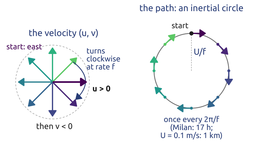
With \(u\) eastward and \(v\) northward, \(\mathbf{k}\times\mathbf{u} = (-v, u)\), so a parcel moved by the Coriolis force alone obeys \[ \frac{du}{dt} = f\,v, \qquad \frac{dv}{dt} = -f\,u \] (Cushman-Roisin and Beckers 2011, sec. 2.3). Starting eastward with speed \(U\), \(u = U\cos ft\) and \(v = -U\sin ft\): the velocity keeps its size and turns clockwise (northern hemisphere) at the rate \(f\), and the parcel runs round a circle of radius \(U/f\) every \(2\pi/f\), an inertial oscillation (Figure 19). At Milan, 0.1 m/s gives circles of about 1 km every 17 h, half the pendulum’s period (Persson 1998, 1377); drifting buoys draw such loops in the ocean.
19 Ferrel (1856–58): wind along the isobars
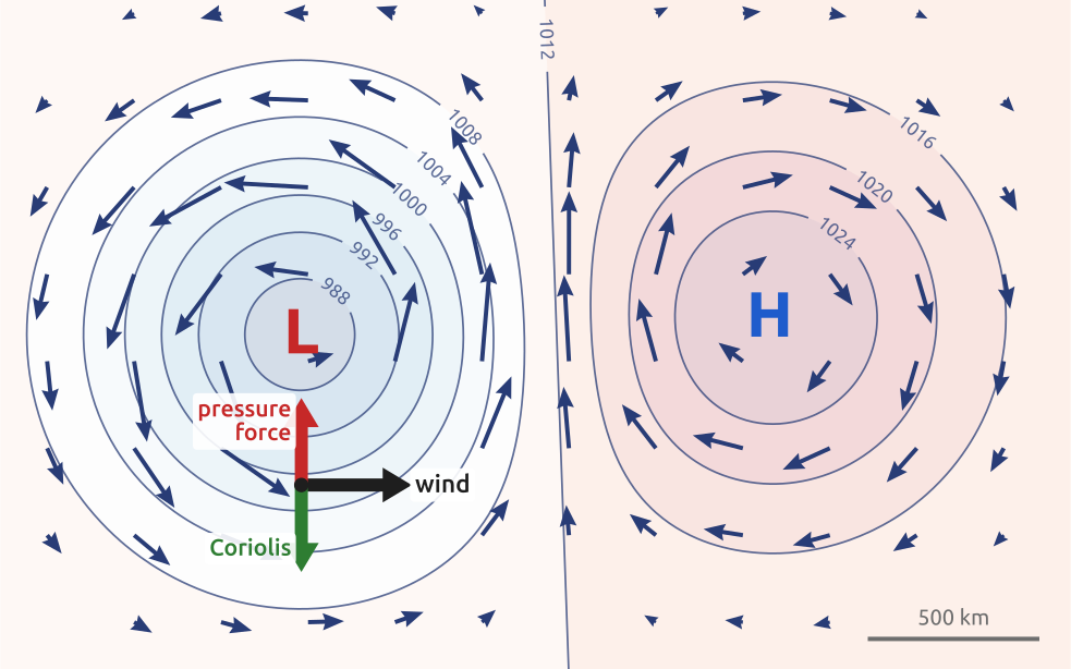
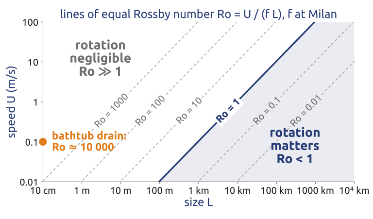
William Ferrel, a reader of Newton and Laplace, concluded in 1856 that the wind blows along the isobars (lines of equal pressure), not from high to low pressure, and in 1858 gave the deflection for motion in any direction (Ferrel 1858; Persson 1998, 1376). With the pressure force, \[ \frac{du}{dt} = f\,v - \frac{1}{\rho}\frac{\partial p}{\partial x}, \qquad \frac{dv}{dt} = -f\,u - \frac{1}{\rho}\frac{\partial p}{\partial y} \] (\(x\) east, \(y\) north); when the forces balance, the wind is geostrophic, \(u_g = -\frac{1}{\rho f}\frac{\partial p}{\partial y}\), \(v_g = \frac{1}{\rho f}\frac{\partial p}{\partial x}\) (Vallis 2017, sec. 2.8.2): along the isobars, anticlockwise around a low in the northern hemisphere, faster where the isobars are closer (Figure 20). Buys Ballot found the rule in weather data in 1857: in the northern hemisphere, with the wind at your back, low pressure is on your left. A sea breeze, small and short-lived, blows from high to low pressure: the rotation has no time to act. The measure is the Rossby number \(Ro = U/(fL)\), the rotation time \(1/f\) over the time \(L/U\) to cross a motion of speed \(U\) and size \(L\); rotation matters when \(Ro \lesssim 1\) (Vallis 2017, sec. 2.8.1; Cushman-Roisin and Beckers 2011, sec. 4.5, who write \(U/(\Omega L)\)).
20 In class: does it feel the Earth’s rotation?
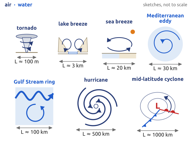
Exercise 2 — Does it feel the Earth’s rotation? For each phenomenon, estimate a typical speed \(U\) and size \(L\), then the Rossby number \(Ro = U/(fL)\), with \(f = 2\Omega\sin\varphi\) and \(\Omega \approx 7.29\times10^{-5}\,\mathrm{s^{-1}}\). Start with \(f\) at Milan (\(\varphi = 45.5^\circ\) N). Rotation matters when \(Ro \lesssim 1\).
The phenomena (Figure 21): sea breeze; lake breeze (Como); tornado; hurricane; mid-latitude cyclone; Gulf Stream ring; Mediterranean mesoscale eddy. Figure 22 is the slide’s diagram.
To hand in: nearer the equator. Redo it for a place of your choice between the equator and \(15^\circ\) (north or south). At what latitude does a mid-latitude cyclone (\(U = 10\) m/s, \(L = 1000\) km) reach \(Ro = 1\)?
21 Observing the ocean, 1769–1876
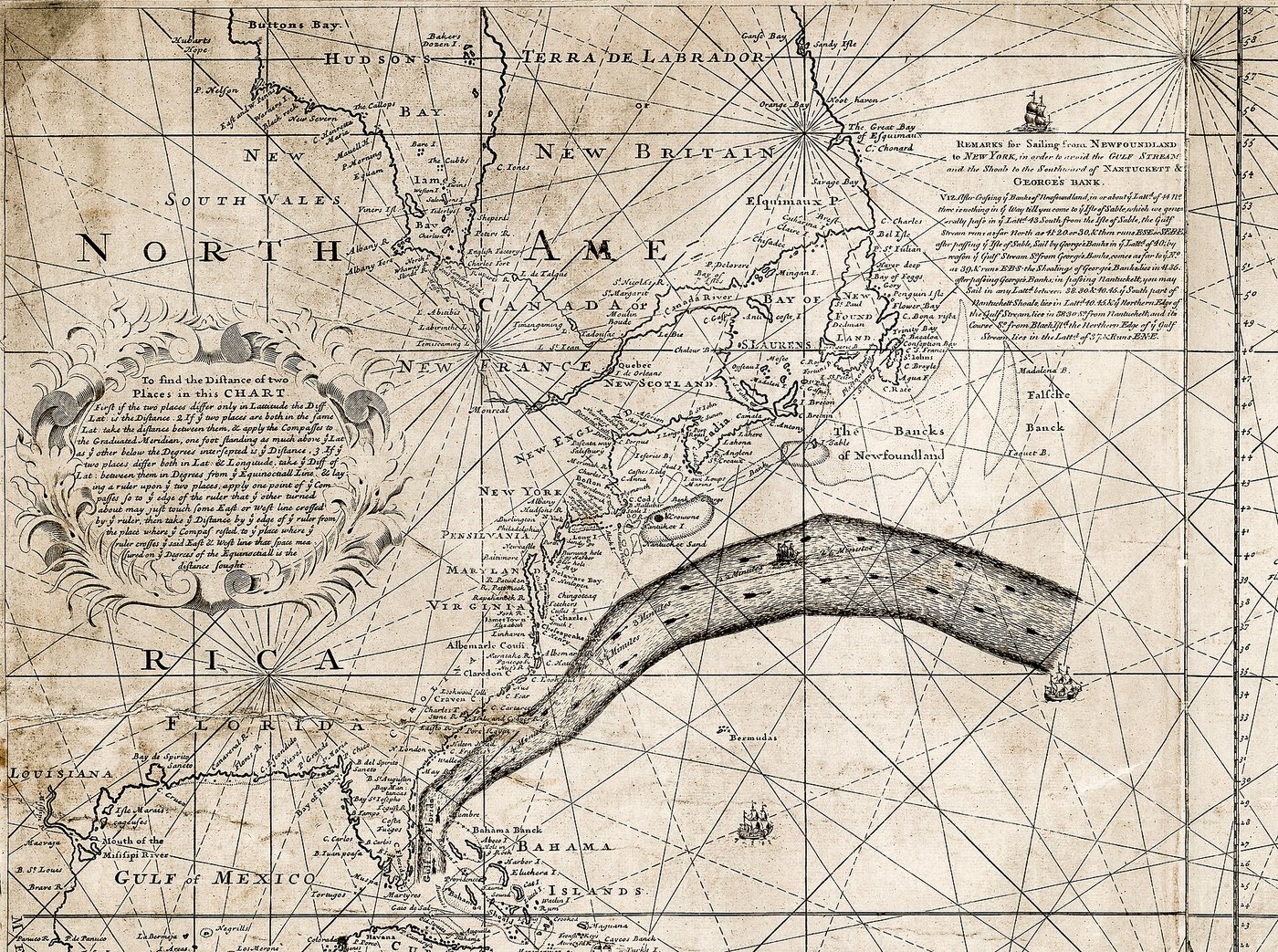
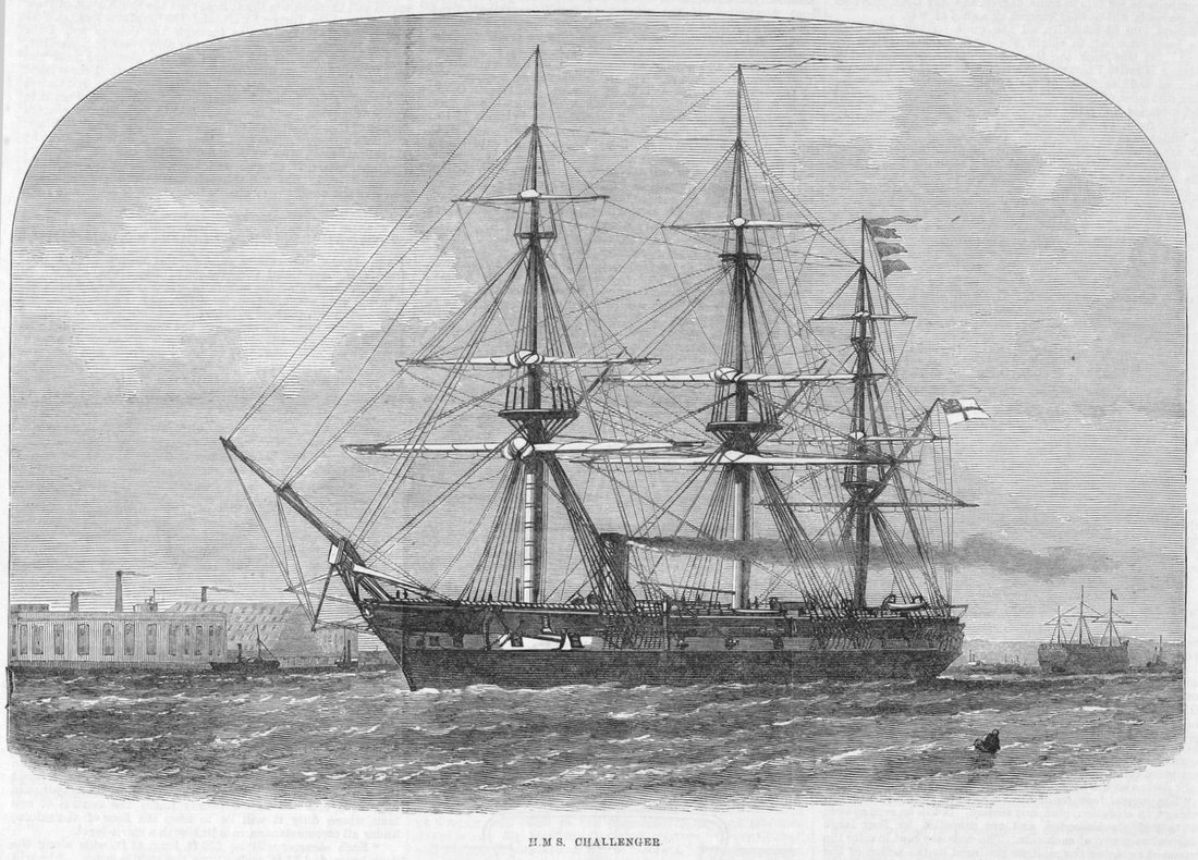
Benjamin Franklin, deputy postmaster of the American colonies, learned that mail ships from England took “a fortnight longer” to cross than merchant ships (Franklin 1786, 314–15); his cousin Timothy Folger, a Nantucket captain, explained that they sailed against the Gulf Stream and drew it, and Franklin printed the chart in London in 1769 (Figure 23) (Stewart 2008, sec. 2.3). From 1847 Matthew Fontaine Maury, of the U.S. Navy, compiled charts of winds and currents from ships’ logs (Maury 1855). HMS Challenger (1872–1876, Figure 24) made the first survey of the deep ocean and found cold water at depth everywhere, even in the tropics (Warren 1981). What drives the currents was disputed: density differences, said William Carpenter; the wind, said James Croll (Warren 1981, sec. 1.2). Both were partly right (Section 23, Section 26).


22 Kelvin (1869): circulation, the spin of a fluid
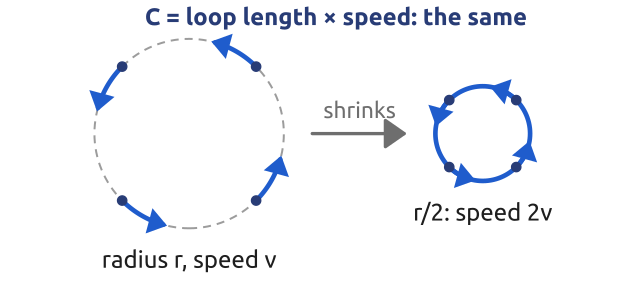
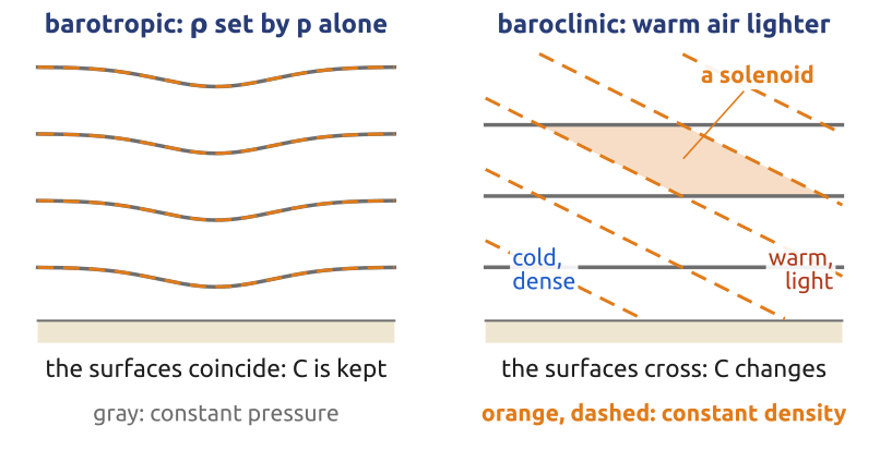
The spin of a fluid is its vorticity \(\boldsymbol{\omega} = \nabla\times\mathbf{u}\), twice the local rate of rotation; Hermann von Helmholtz (1858) showed that without friction vortex lines move with the fluid (Helmholtz 1858). William Thomson (Lord Kelvin) used the circulation around a closed curve with line element \(d\mathbf{l}\), bounding a surface \(A\), \[ C = \oint \mathbf{u}\cdot d\mathbf{l} = \int_A \boldsymbol{\omega}\cdot d\mathbf{A}, \] and proved that, at constant density and without friction, \(DC/Dt = 0\) around a curve moving with the fluid (read 1867, printed 1869) (Thomson 1869; Thorpe et al. 2003, 472); Ludwik Silberstein (1896) extended it to barotropic fluids, whose density depends on pressure alone, and showed that this condition is also necessary. The textbooks state Kelvin’s theorem in this barotropic form (Vallis 2017, sec. 4.3.2; Holton 2004, sec. 4.1). A ring of radius \(r\) turning at speed \(V\) has \(C = 2\pi r V\): shrunk to half the radius, it turns twice as fast (Figure 25 (a)). But then a barotropic fluid at rest stays at rest. In air and sea, at equal pressure, warm air is lighter than cold, and warm or fresh water lighter than cold or salty: the surfaces of constant pressure and density cross, and the fluid is baroclinic (Figure 25 (b)).
23 Bjerknes (1898): how winds and currents start
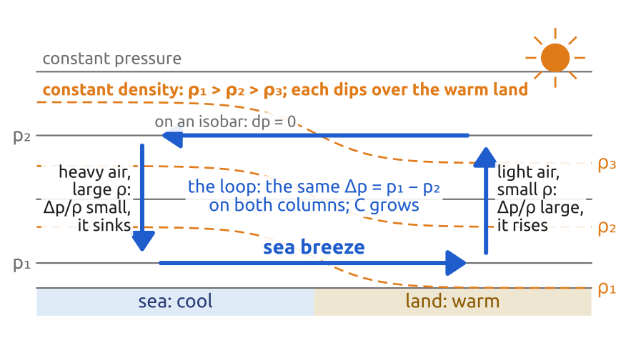
Silberstein (1896) and Vilhelm Bjerknes (1898) extended Kelvin’s theorem to baroclinic fluids, the baroclinic circulation theorem [Vallis (2017), §4.3.2; sometimes called the Bjerknes or Bjerknes–Silberstein theorem]: \[ \frac{DC}{Dt} = -\oint \frac{dp}{\rho} , \] non-zero where the surfaces of constant pressure and density cross. Silberstein found it first, as mathematics; Bjerknes, citing him, used it for breezes, monsoons, trade winds, cyclones and ocean circulations (Bjerknes 1898; Thorpe et al. 2003, 473–76). For the sea breeze (Figure 26), take a loop along two isobars, \(p_1\) near the ground and \(p_2\) aloft, closed by columns over the warm land and over the sea. Along the isobars \(dp = 0\); both columns span \(\Delta p = p_1 - p_2\), and per kilogram the push is \(\Delta p/\rho\), larger for the light air: \[ \frac{DC}{Dt} = \Delta p\left(\frac{1}{\rho_{\mathrm{land}}} - \frac{1}{\rho_{\mathrm{sea}}}\right) > 0 \] (\(1/\rho\) averaged over each column): air rises over the land, and a breeze blows from the sea. The same mechanism drives Carpenter’s density-driven ocean circulation. In 1902 Bjerknes added the Earth’s rotation (Thorpe et al. 2003, 476–77); the result was given by Poincaré in 1893 (Vallis 2017, Ch. 4, endnote 4).
24 Teisserenc de Bort, Assmann (1902): layers
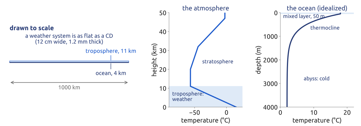
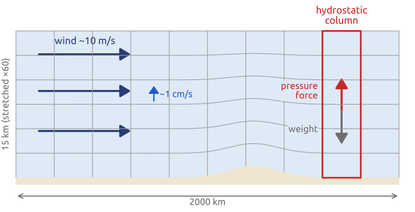
In 1902 Léon Teisserenc de Bort and Richard Assmann, from balloon soundings, found that the air stops cooling with height above about 11 km, and higher up warms: the troposphere, where weather happens, lies under the stratosphere (Vallis 2017, Ch. 15, endnote 7, p. 583). The ocean is layered too: warm, light water over a cold abyss. Both are thin: a weather system 1000 km wide and 10 km deep is as flat as a compact disc (1/100), an ocean basin 5000 km wide and 4 km deep flatter still (about 1/1000) (Figure 27). Motion is mostly horizontal (winds of 10 m/s, vertical velocities of cm/s), and each column is close to hydrostatic balance (Vallis 2017, sec. 2.7; Cushman-Roisin and Beckers 2011, sec. 4.3).
25 Bjerknes (1904): an initial-value problem
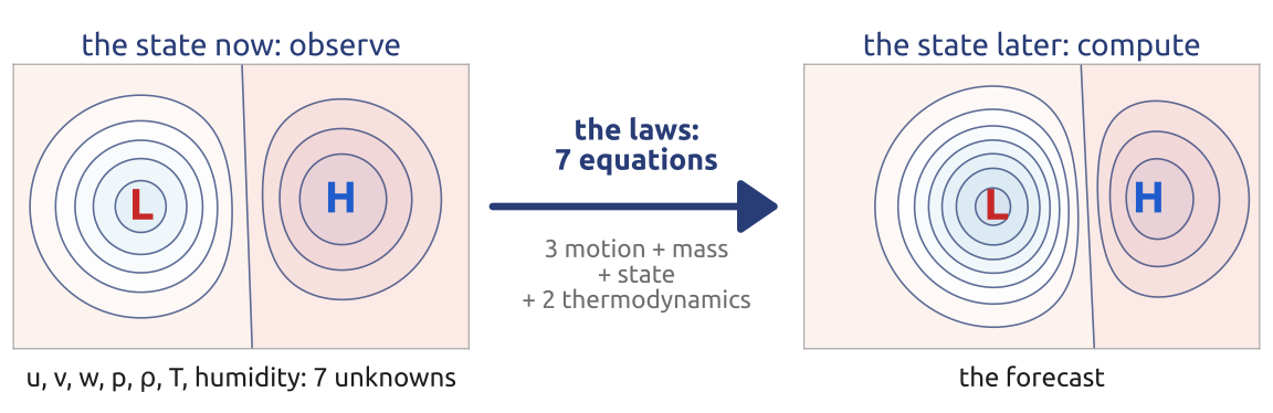
Bjerknes (1904) posed forecasting as a problem of physics, needing “the state of the atmosphere at a given time” and “the laws according to which one state of the atmosphere develops from another” (Bjerknes 1904, transl. p. 663). He counted seven variables (three velocity components, pressure, density, temperature, humidity) and seven equations (three of motion, mass, the equation of state, two laws of thermodynamics) (Bjerknes 1904, transl. p. 664); as Lynch notes, the seventh should be the conservation of water rather than the second law (Lynch 2008b, sec. 1.1), as it is today (Section 40). A forecast is then an initial-value problem (Figure 28): observe the state (“diagnosis”), integrate forward (“prognosis”); Cleveland Abbe had said much the same in 1901 (Abbe 1901). As “there can be no question of a strictly analytical integration” (transl. p. 664), Bjerknes proposed graphical methods (Lynch 2008b, sec. 1.1); his Bergen school built modern weather analysis (fronts, air masses).
26 Ekman (1905): the wind-driven ocean
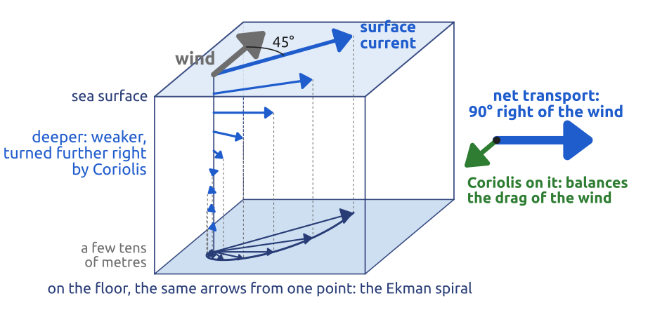
On the Fram (Arctic, 1893–96) Fridtjof Nansen saw the ice drift \(20\)–\(40^\circ\) to the right of the wind (Nansen 1902; Stewart 2008, sec. 9.2). In 1900 Nansen shared his intuition about wind-driven currents with Bjerknes; Bjerknes’ student Vagn Walfrid Ekman, called into the discussion, “produced the theory of the Ekman spiral that very evening” (Munk 2002, 136). In a steady state the internal friction of the wind-driven layer cancels out, so only the Coriolis force, perpendicular to the layer’s motion, can balance the drag of the wind: the layer moves at right angles to the wind (to the right in the northern hemisphere), with volume transport per unit width \[ \mathbf{M}_E = \frac{\boldsymbol{\tau}\times\mathbf{k}}{\rho_0 f} , \] \(\boldsymbol{\tau}\) being the wind stress (force per unit area) and \(\rho_0\) the density of sea water, whatever the friction (Ekman 1905); multiplied by \(\rho_0\) it is the mass transport \(\mathbf{M}_E\) of Vallis (Vallis 2017, sec. 5.7), and its components are the \((U, V)\) of Cushman-Roisin and Beckers (Cushman-Roisin and Beckers 2011, sec. 8.5). With constant turbulent mixing the surface current is \(45^\circ\) right of the wind, and deeper water slower and turned further, the Ekman spiral (Figure 29). Observed angles are smaller than \(45^\circ\), because the turbulent mixing is not constant with depth (Cushman-Roisin and Beckers 2011, Sect. 8.7); Nansen’s ice, moving with the surface water, turned 20–\(40^\circ\). Where Ekman transports converge or diverge, water is pushed down or drawn up: the start of the theory of the gyres.
27 Richardson (1922): the laws, by numbers
Lewis Fry Richardson took Bjerknes’ programme literally. During the First World War, partly while an ambulance driver in France, he put the hydrostatic primitive equations (Section 41) on a grid over Europe (Figure 30; columns about 200 km apart, five layers), replaced derivatives by finite differences, and computed by hand the six-hour change from the observations of 20 May 1910 (Richardson 1922), with a three-hour time step (Lynch 1999). The 23 computing forms (Lynch 2008b) took about six weeks of computing, “on a heap of hay in a cold wet rest billet”, spread over some two years (Hunt 1998; Lynch 1999, 61–68).
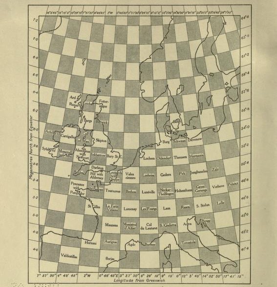
28 Richardson’s dream: the forecast factory
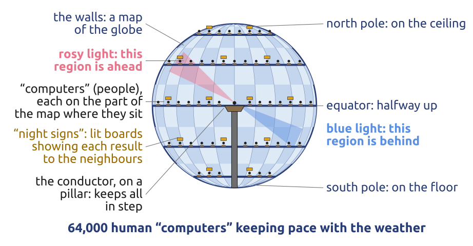
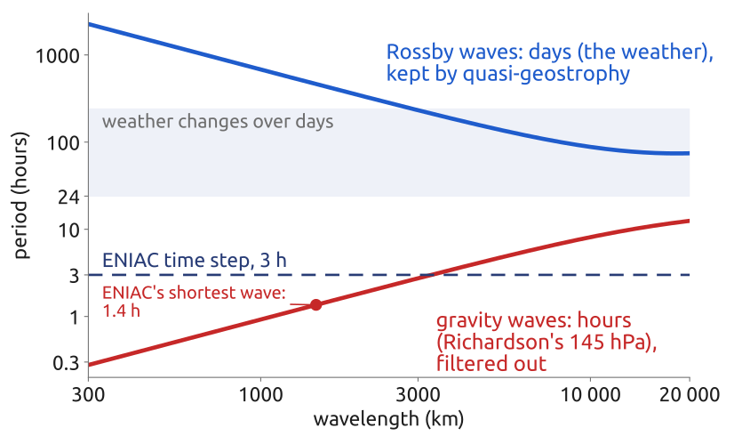
The forecast gave “145 millibars in 6 hours, whereas observations show that the barometer was nearly steady” (Richardson 1922, 187). His equations carry fast gravity waves, with periods of hours; observed winds and pressures are slightly out of the balance (roughly geostrophic) kept by the slow weather, and the imbalance sets off large gravity-wave tendencies. Peter Lynch redid the computation: the same 145 hPa, but under 1 hPa once the initial state was balanced (an initialization) (Lynch 1999; 2008b, secs. 1.2–1.3). Further steps would have failed too: a step must not let the fastest wave cross more than about one grid interval (Courant, Friedrichs and Lewy, 1928), and three hours was too long (Vallis 2017, Ch. 11, note 4, p. 442). Near its end the book imagines a “forecast factory” of 64,000 human computers led by a conductor (Figure 31) (Richardson 1922, 219), which Lynch calls an early example of massively parallel processing (Lynch 2008b); its preface had said: “Perhaps some day in the dim future it will be possible to advance the computations faster than the weather advances […] But that is a dream” (Richardson 1922, vii). Stephen Conlin’s painting of the factory (1986, copyrighted) is on Lynch’s page: maths.ucd.ie: Richardson’s Forecast Factory.
29 Rossby (1939): waves in the mid-latitude winds
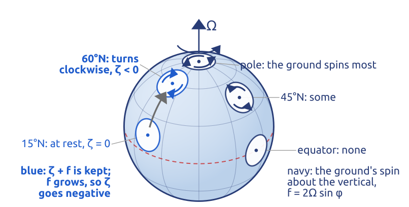
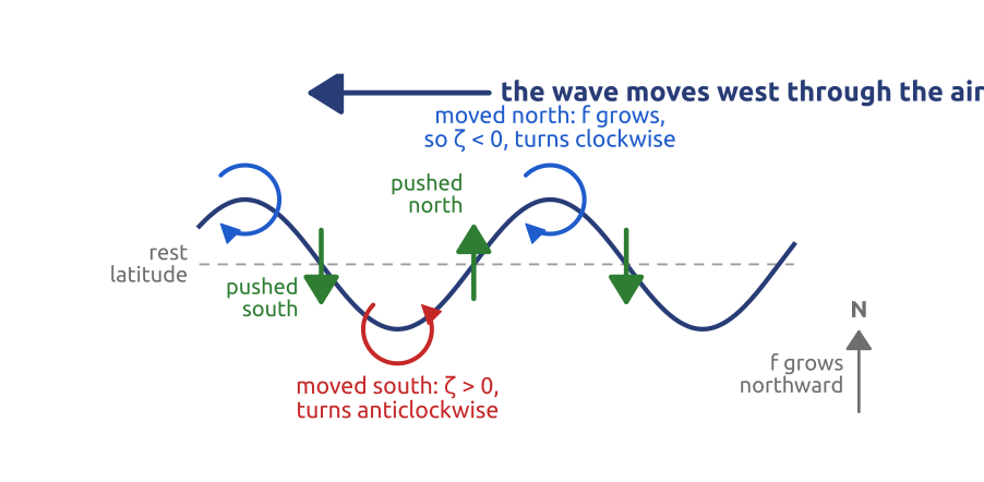
On the rotating Earth, Kelvin’s theorem holds for the circulation seen from the stars (Poincaré, 1893; Bjerknes, 1902) (Thorpe et al. 2003; Vallis 2017, Ch. 4, endnote 4). With \(\zeta = \partial v/\partial x - \partial u/\partial y\) the vertical vorticity relative to the ground (positive anticlockwise seen from above), a small disk of area \(A\) has absolute circulation \((\zeta + f)A\); if \(A\) is kept, \[ \frac{D}{Dt}(\zeta + f) = 0 , \] the barotropic vorticity equation: a disk moving north meets a larger \(f\) and turns clockwise (Figure 32). Carl-Gustaf Rossby used it in 1939 (Rossby and collaborators 1939; Vallis 2017, secs. 6.4.2–6.4.3) with \(f \approx f_0 + \beta y\), \(y\) northward, \(\beta = df/dy = 2\Omega\cos\varphi/a\) (\(1.6\times10^{-11}\ \mathrm{m^{-1}\,s^{-1}}\) at \(45^\circ\)N; positive in both hemispheres). In a wave, air pushed north turns clockwise and air pushed south anticlockwise, shifting the pattern west (Figure 33). For wavenumber \(k = 2\pi/L\) in an eastward wind \(U\) the speed over the ground is \[ c = U - \frac{\beta}{k^2} . \] With \(U = 15\) m/s at \(45^\circ\)N, a 4000 km wave moves east at about 8 m/s, waves of about 6000 km stand still, longer ones drift west: cyclones travel east though the waves drift west through the air. Hough had met these waves in Laplace’s tidal equations (1897–98) (Vallis 2016, 5). In the ocean, with no strong eastward current to carry them, they cross the Pacific westward in about 200 days near the equator (Vallis 2017, 892) and in about a decade at mid-latitudes (Jacobs et al. 1994; Chelton and Schlax 1996).
30 Rossby waves on the jet: August 2002
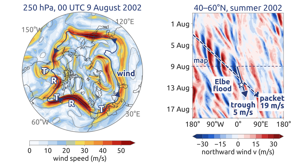
On upper-air maps the wind blows nearly along the height contours of a pressure surface, higher heights on its right (northern hemisphere); the contours bend into ridges and troughs (Ahrens 2005, 145–46), clearest near the tropopause, in the jet stream. Figure 34 shows the wave packet of early August 2002, the running example of Wirth et al. (2018), in ERA5, a reanalysis (past weather reconstructed from observations with a forecast model) (Hersbach et al. 2020). Its right panel is a Hovmöller diagram, longitude against time, after Ernest Hovmöller, who drew them by hand (Hovmöller 1949). Troughs move east at 1–6 m/s, slower than the 16 m/s mean wind: through the air they drift west. The packet runs east at about 19 m/s, from the date line on 3 August to \(90^\circ\)E on 15 August, new troughs growing at its front (Wirth et al. 2018, 1966–72): it moves at the group velocity, in the simplest theory \(c_g = U + \beta/k^2\), while the troughs move at \(c = U - \beta/k^2\) (Rossby 1945; Holton 2004, sec. 7.7.1). Over Europe it brought the low of the Elbe flood: 312 mm of rain in 24 h at Zinnwald on 12–13 August, the Elbe at Dresden highest since 1275 (Ulbrich et al. 2003b, 434–35; 2003a, 371).
31 Blocks: when a Rossby wave stands still
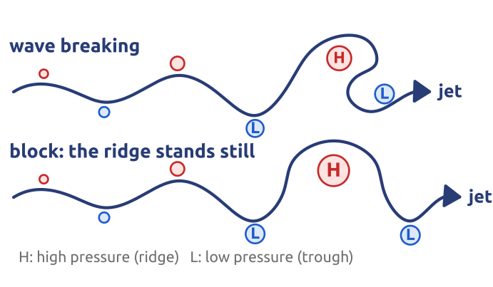
A Rossby wave can grow until its crest overturns (breaking), or until a large ridge stalls for days or weeks with the jet going around it: a block (Figure 35) (Holton 2004, sec. 10.6), an omega block when the contours draw an \(\Omega\) (Woollings et al. 2018). Summer blocks bring heat waves (Ahrens 2005, 356), winter blocks over the North Atlantic cold to Europe (Sillmann et al. 2011). For small amplitudes a wave stands still when \(c = U - \beta/k^2 = 0\), at the wavelength \(L_s = 2\pi\sqrt{U/\beta}\) (Holton 2004, sec. 7.7.1, eq. 7.93, no north–south wavenumber): about 5200 km for \(U = 10\) m/s at \(50^\circ\)N (\(\beta = 1.47\times10^{-11}\ \mathrm{m^{-1}\,s^{-1}}\)), the size of a block. Breaking and blocking are nonlinear; the linear formula only says that such waves can stand still.
32 Blocking over Europe: summer 2026
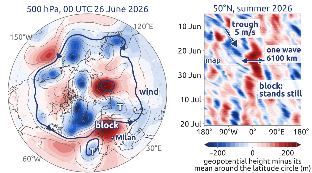
In ERA5 (Figure 36) a ridge stood over western Europe at \(50^\circ\)N, between \(15^\circ\)W and \(22^\circ\)E, from 17 June to 9 July 2026; on 26 June the 5760 m contour at 500 hPa drew an omega around it. The Copernicus Climate Change Service tied western Europe’s record June–July temperatures, \(2.79\,^\circ\)C above the 1991–2020 average, to this “atmospheric blocking”, which drew hot air north from Africa (Copernicus Climate Change Service 2026c); the summer was the warmest on record there (Copernicus Climate Change Service 2026b), with record or near-record low flows of the Po, the Rhine and the Danube (Copernicus Climate Change Service 2026a). The mean eastward wind at 500 hPa and \(50^\circ\)N over the block’s life, \(U \approx 8.5\) m/s, gives \(L_s \approx 4800\) km, against a block wave of about 6100 km: same scale, not the same number. The formula ignores the wave’s north–south extent (\(k^2 + l^2 = \beta/U\), \(l\) the north–south wavenumber), the change of wind with height and the large amplitude. Blocks seem to be maintained by the smaller disturbances fed into them (Holton 2004, sec. 10.6); their life cycle still lacks a complete theory (Woollings et al. 2018).
33 Charney (1948): keep the slow waves only
Jule Charney estimated the size of each term of the equations at large scales (scale analysis) (Charney 1948; Lynch 2008b, sec. 2.2): there the wind is nearly geostrophic and the air nearly hydrostatic, and simplifying with these balances removes the gravity waves and keeps the slow motions. For one layer the quasi-geostrophic equation keeps the potential vorticity, \[ \frac{D}{Dt}\Big(\zeta + f - \frac{\psi}{L_d^2}\Big) = 0 , \] with \(\psi\) the streamfunction (\(u = -\partial\psi/\partial y\), \(v = \partial\psi/\partial x\), \(\zeta = \nabla^2\psi\)) and \(L_d = c/f\) the deformation radius, \(c\) the gravity-wave speed: about 3000 km for one layer as deep as the atmosphere (\(c \approx 300\) m/s); the internal radius of the stratified atmosphere, \(L_d = NH/f\) with \(N\) the buoyancy frequency and \(H\) the depth, the size of weather systems, is about 1000 km. At scales much smaller than \(L_d\) Rossby’s equation remains. Linear one-layer gravity waves have \(\omega^2 = f^2 + c^2k^2\) (hours), Rossby waves \(\omega = -\beta k/(k^2 + L_d^{-2})\) (days; the minus: westward), \(\omega\) being the frequency (Figure 37); the filtered equation keeps only the second, and allows long time steps. Still, the four 24-hour forecasts of 1950 took about 1,000,000 multiplications and divisions and 100,000 punched cards (Charney et al. 1950, 245): a job for a machine.
34 The first computer forecast (1950)
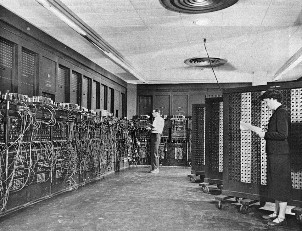
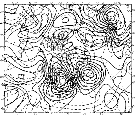
John von Neumann, a consultant at Los Alamos from 1943, came out of the war convinced of machine computing (Lewis 2021); the ENIAC (Electronic Numerical Integrator and Computer), built for the U.S. Army, began in December 1945 with “an urgent problem from Los Alamos” (Platzman 1979). In Princeton he chose weather as the scientific problem for his own new computer; the Navy funded his Meteorology Project in 1946, led by Charney from 1948 (Thompson 1983; Lynch 2008b). In March 1950, on the ENIAC at Aberdeen, Maryland (Figure 38), Charney, Ragnar Fjørtoft and von Neumann integrated the barotropic vorticity equation for the 500 hPa level, \[ \frac{\partial}{\partial t}\nabla^2\psi + J(\psi, \nabla^2\psi + f) = 0, \] with the Jacobian \(J(a,b) = \partial_x a\,\partial_y b - \partial_y a\,\partial_x b\), the advection of \(b\) by the flow of streamfunction \(a\); each step solves a Poisson problem for \(\partial\psi/\partial t\). On \(15\times18\) grid intervals of 736 km, steps of 1, 2 and 3 h gave nearly the same, stable results; a 24-hour forecast took about 24 hours (Charney et al. 1950, 244–45; Lynch 2008a). The forecast from 30 January 1949 was good (Figure 39), that from 5 January poor; operational forecasts followed within a few years.

35 Sverdrup, Stommel, Munk: the wind-driven gyres
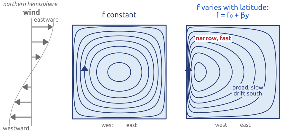
Harald Sverdrup (1947) combined the Ekman transport with \(\beta\): below the surface layer the interior drifts north or south so that its change of \(f\) balances the spin put in by the wind, \[ \beta V = \frac{\mathbf{k}\cdot\nabla\times\boldsymbol{\tau}}{\rho_0} , \] with \(V\) the northward transport per unit width and \(\mathbf{k}\cdot\nabla\times\boldsymbol{\tau}\) the vertical component of the curl of the wind stress, its spin (Sverdrup 1947; Vallis 2017, sec. 19.1). Eastward winds to the north and westward trade winds to the south spin the subtropical ocean clockwise; the interior drifts south. Henry Stommel (1948), with a rectangular ocean and bottom friction, showed that the return flow is a narrow, fast current on the western side, because of \(\beta\) alone (Stommel 1948) (Figure 40). Walter Munk (1950), with lateral friction and the observed winds, obtained the main gyres with transports of the right size (Munk 1950; Wunsch 2021). The same \(\beta\) sends the atmosphere’s waves west and presses the return flow of the gyres against the western side of the ocean.
36 Bryan, Cox (1960s): the ocean by numbers
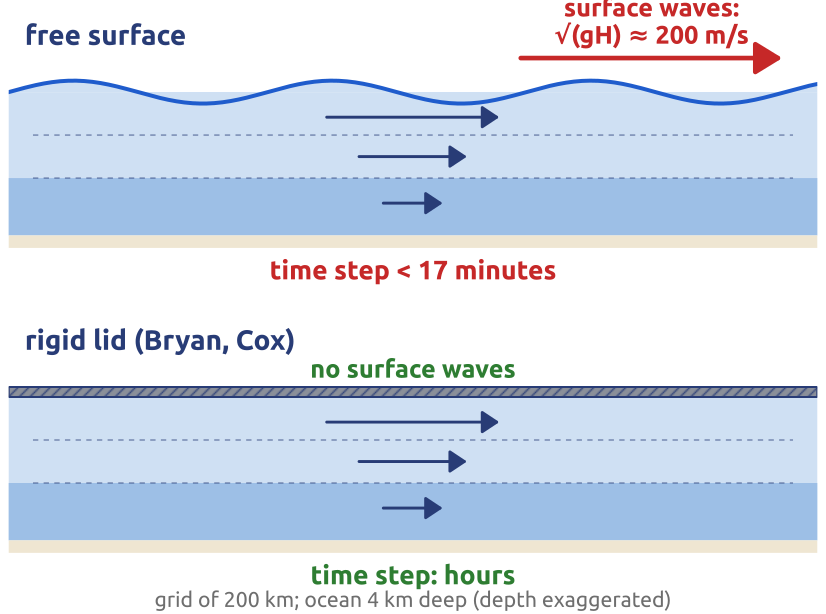
At the Geophysical Fluid Dynamics Laboratory (GFDL), Joseph Smagorinsky hired Kirk Bryan in 1960 to build a model of the world ocean, “a fool’s mission” to many (Randall et al. 2019, sec. 4a). With the programmer Michael Cox, Bryan had a model by the mid-1960s and published the method in 1969, for the primitive equations of the ocean (Bryan 1969, 349–51): \[ \begin{gathered} \frac{D\mathbf{u}_h}{Dt} + f\,\mathbf{k}\times\mathbf{u}_h = -\frac{1}{\rho_0}\nabla_h p + \mathbf{F}, \qquad \frac{\partial p}{\partial z} = -\rho g, \qquad \nabla\cdot\mathbf{u} = 0,\\ \frac{DT}{Dt} = \dot T, \qquad \frac{DS}{Dt} = \dot S, \qquad \rho = \rho(T, S, p), \end{gathered} \] for the horizontal current \(\mathbf{u}_h\) (\(\nabla_h\): horizontal gradient), temperature \(T\) and salinity \(S\), with friction \(\mathbf{F}\) and turbulent mixing \(\dot T\), \(\dot S\) (the dot names the source of a property carried by the fluid, not a time derivative (Vallis 2017, sec. 1.2, eq. 1.41)); the Boussinesq approximation keeps density changes only in the weight (\(\rho_0\): mean density). The key device was a rigid lid, a flat top (\(w = 0\)) that removes the surface gravity waves (about 200 m/s) and permits long time steps (Figure 41), as Charney’s filter did for the air. In 1969 Syukuro Manabe and Bryan coupled it to an atmosphere model, “the first true climate model” (Manabe and Bryan 1969; Randall et al. 2019): 5 ocean levels, a 500 km grid, an idealized basin (Manabe and Bryan 1969, 786–87). Manabe shared the 2021 Nobel Prize in Physics.
37 Timeline: to weather and ocean models
By the 1960s (Figure 42) air and sea were understood as fluids obeying Newton’s laws (Euler, Navier, Stokes) on a rotating Earth (Coriolis), in thin, nearly hydrostatic and geostrophic layers (Laplace, Ferrel), whose spin is made by density differences and otherwise kept (Kelvin, Bjerknes), with \(f\) growing northward (Rossby, Stommel). Forecasting was an initial-value problem (Bjerknes), solvable by numbers once the fast waves were controlled (Richardson, Courant, Charney): a computer did it in 1950, the ocean followed, and the first coupled model came in 1969 (Vallis 2016; Lynch 2008b).
38 A weather model today
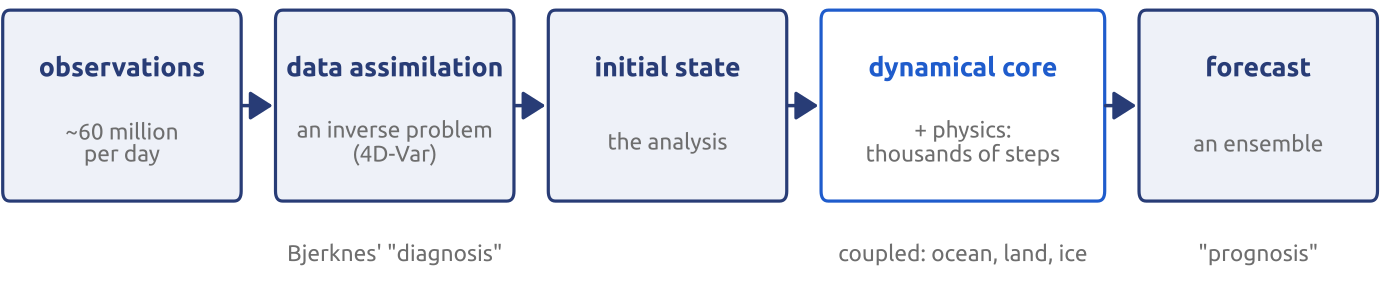
A forecast today follows Bjerknes’ plan and Richardson’s method (Figure 43) (Kalnay 2003, Ch. 1). Data assimilation combines observations with a short forecast into the initial state; the dynamical core steps the fluid equations forward on the grid; parameterizations add what the grid cannot resolve (radiation, clouds, turbulence); ocean, land and ice enter as forcings or coupled models; and the forecast, an ensemble, is the first guess of the next cycle. In 1950: one equation, one layer, a 736 km grid, a day of computing per day of forecast; today: the full equations on the globe, about 10 km and 100 levels, minutes of computing per day (see Bauer et al. 2015). Lynch finds today’s algorithms “remarkably similar to Richardson’s scheme” (Lynch 2008b, sec. 1.2).
39 Operational weather forecast model
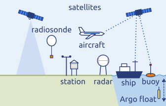
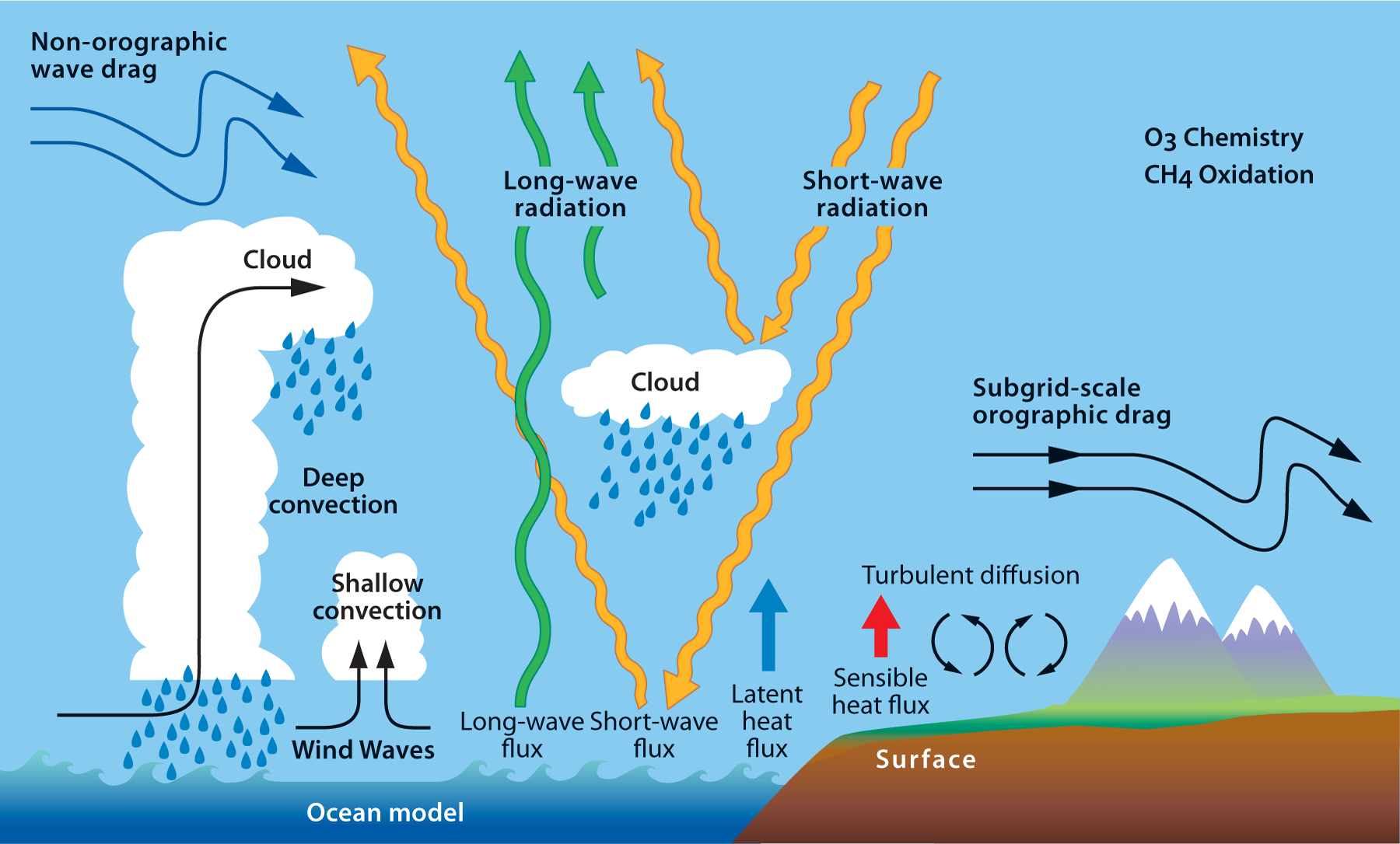
The same chain with real pieces (Figure 44, Figure 45). The data come from the global observing system coordinated by the World Meteorological Organization: satellites in polar and geostationary orbits, radiosondes, aircraft, surface stations, radars, ships, drifting buoys and Argo floats (community.wmo.int: Global Observing System). Assimilation brings them into the model’s variables on its grid: the initial conditions. The dynamical core advances the fluid equations in time; the physics adds, as parameterizations, what the grid cannot resolve: short- and long-wave radiation, clouds and deep convection, turbulent diffusion, the drag of unresolved mountains and gravity waves, ozone chemistry (ecmwf.int: Atmospheric physics). The forcings come from below: sea-surface temperature, sea ice, soil moisture and snow, prescribed or computed by coupled ocean, ice and land models. The forecast of one cycle is the first guess of the next (Kalnay 2003, Ch. 1).
40 The equations of motion
Together, in the frame of the rotating Earth: \[ \begin{gathered} \frac{D\mathbf{u}}{Dt} + 2\boldsymbol{\Omega}\times\mathbf{u} = -\frac{1}{\rho}\nabla p - \nabla\Phi + \nu\nabla^2\mathbf{u},\\ \frac{D\rho}{Dt} + \rho\,\nabla\cdot\mathbf{u} = 0, \qquad p = \rho R T,\\ c_p\frac{DT}{Dt} - \frac{1}{\rho}\frac{Dp}{Dt} = Q, \qquad \frac{Dq}{Dt} = \dot q , \end{gathered} \] seven equations for \(u, v, w, p, \rho, T, q\): Bjerknes’ programme (Bjerknes 1904, transl. p. 664; Vallis 2017, secs. 1.2–1.6, 2.1). Here \(\mathbf{u} = (u, v, w)\), \(\Phi\) includes the centrifugal force, \(q\) is the specific humidity (water vapour per unit mass of air) and \(\dot q\) its sources and sinks (evaporation, condensation; a source, not a time derivative); the mass equation is Euler’s, written with \(D/Dt\). Each term has its giant: Newton and Euler, Coriolis, Torricelli, Navier and Stokes, Boyle, Charles and Gay-Lussac, Clausius. In the ocean, salinity replaces humidity, and an empirical equation of state of seawater the gas law.
41 A preview: the primitive equations
For thin shells (Vallis 2017, secs. 2.2.4, 2.7) the vertical momentum equation becomes the hydrostatic balance, and only \(f\), the local vertical part of the rotation, is kept: \[ \frac{D\mathbf{u}_h}{Dt} + f\,\mathbf{k}\times\mathbf{u}_h = -\frac{1}{\rho}\nabla_h p + \mathbf{F}, \qquad \frac{\partial p}{\partial z} = -\rho g , \] with \(\mathbf{u}_h = (u, v)\), \(\nabla_h\) the horizontal gradient, \(\mathbf{F}\) friction, and mass, heat and state as before: the primitive equations (Figure 46). Richardson solved them by hand (Richardson 1922); most twentieth-century global weather and climate models solved them, and ocean models (with Boussinesq) still do. At grid spacings of a few kilometres, where the vertical accelerations of convection matter, models return to the full equations.
42 Key points
- The local rotation is \(f = 2\Omega\sin\varphi\), about \(10^{-4}\ \mathrm{s^{-1}}\) at Milan: moving air and water turn right in the northern hemisphere, left in the southern.
- Geostrophic balance: the large-scale wind blows along the isobars, with low pressure on its left in the northern hemisphere.
- The Rossby number \(Ro = U/(fL)\): the rotation matters when \(Ro \lesssim 1\).
- Spin: circulation and vorticity. Density differences create it; otherwise \(\zeta + f\) is kept, and \(f\) grows northward (\(\beta\)): Rossby waves drift west, and the gyres are pressed against the west.
- A forecast is an initial-value problem; fast waves and balance decide whether it works.
- The equations: Navier–Stokes on the rotating Earth, with mass, heat and the gas law; thin shells are hydrostatic (the primitive equations).
Further reading
History: Vallis (2016), Lorenz (1983) and Lynch (2008b) (atmosphere); Munk (2002) and Warren and Wunsch (1981) (ocean); Persson (1998) (the Coriolis force).