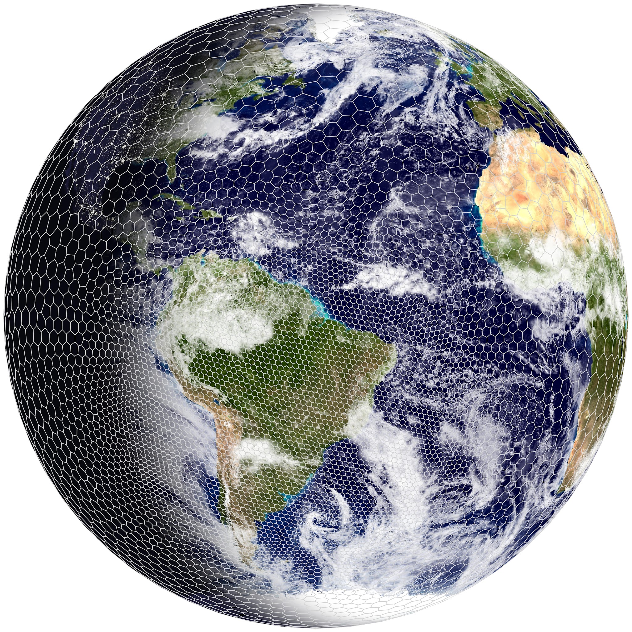
November 2026 · Politecnico di Milano

A historical overview of atmosphere and ocean dynamics

Atmosphere and Ocean Dynamics — Lecture 1

Prof. Dr. Pedro da Silva Peixoto

Applied Mathematics
Instituto de Matemática e Estatística
Universidade de São Paulo

Visiting Professor at MOX Lab
Politecnico di Milano

Atmosphere and ocean dynamics

Atmosphere: cyclones and fronts

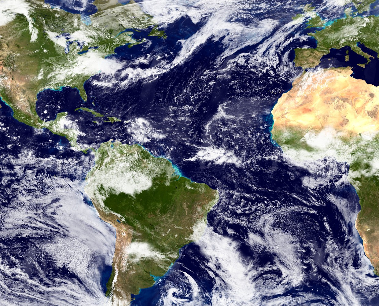Clouds seen by the satellite instrument MODIS: NASA Blue Marble (2002)

Why do the winds blow mostly westward in the tropics, and eastward at higher latitudes?

Ocean: gyres and the Gulf Stream

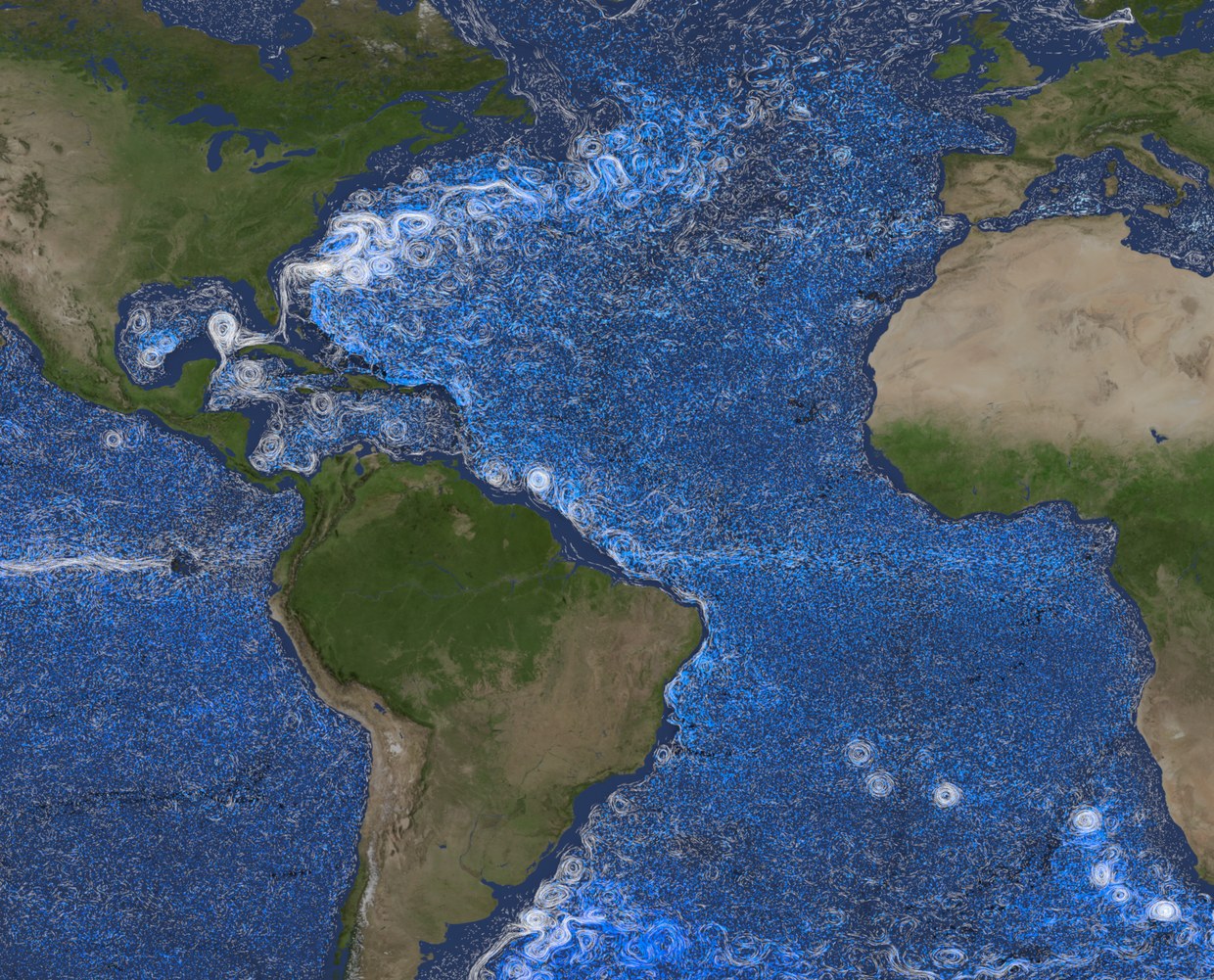Currents from the ECCO2 ocean model: NASA Scientific Visualization Studio

Why is the fast, narrow current on the western side of the Atlantic Ocean, off America and not off Europe?

Can we model and forecast this?

Goals: Understand and model the large-scale motions of thin layers of air and water on a rotating planet

Figures: commons.wikimedia.org: Land_ocean_ice_cloud_hires.jpg (NASA Blue Marble) · svs.gsfc.nasa.gov/5479 (Perpetual Ocean 2)

Same Atlantic sector and scale in both maps: cyclones ~1000 km, ocean eddies ~100 km. No previous lecture: it starts from what the maps show, and the questions of the day.

Scales of motion

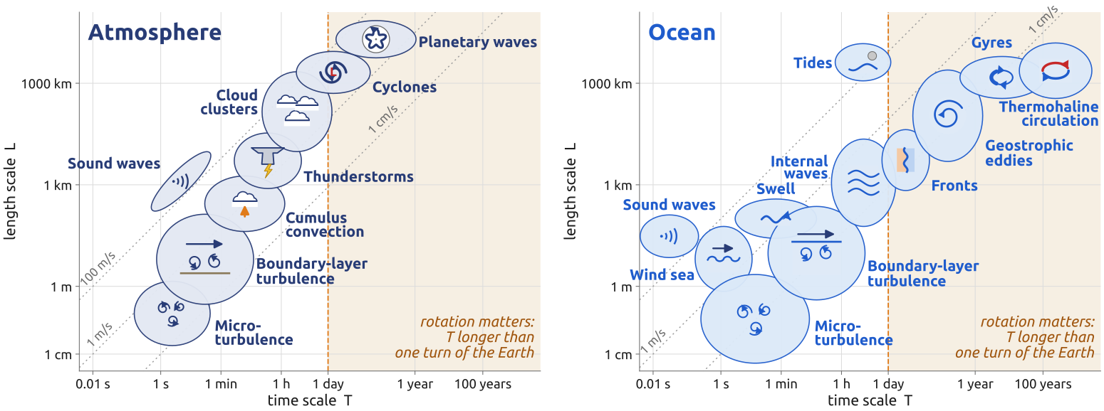
Each ellipse: the typical length \(L\) and time \(T\) of a phenomenon (symbols not to scale); dotted lines: speed \(U = L/T\)

Large motions are slow, and the ocean is about 100 times slower than the air; the Earth’s rotation matters for motions that last longer than a day

Figure redrawn after Fig. 1.7 of Cushman-Roisin and Beckers (2011) (diagram by H. von Storch); text: its sec. 1.5, 1.7 and Table 1.2

Ask first: where would a hurricane go? The Gulf Stream? (Both right of the 1-day line.) Cyclones ~10 m/s, ocean eddies ~1 cm/s: same physics, slower ocean. Rotation: a motion that lasts longer than one turn of the Earth feels it (CR&B eq. 1.2). The course: the right half.

On the shoulders of giants

“If I have seen further it is by standing on the shoulders of Giants.”

Isaac Newton, letter to Robert Hooke, 5 February 1675/6

Torricelli 1643 · Pascal 1648 · Boyle 1662 · Halley 1686 · Newton 1687 · Hadley 1735 · Euler 1755 · Laplace 1776 · Navier 1822 · Carnot 1824 · Coriolis 1835 · Ferrel 1856–58 · Helmholtz 1858 · Kelvin 1869 · Bjerknes 1904 · Ekman 1905 · Richardson 1922 · Rossby 1939 · Sverdrup 1947 · Stommel 1948 · Charney & von Neumann 1950 · Munk 1950

Today: the giants, 1643 → the 1960s: the weight and the spring of the air (Torricelli, Pascal, Boyle) → rotation and the equations of a fluid (Halley to Ferrel) → spin and circulation (Kelvin, Bjerknes) → forecasting by numbers (Bjerknes, Richardson, Rossby, Charney, the ENIAC) → the wind-driven ocean (Ekman to Munk) and the ocean by numbers (Bryan, Cox) → a model today, and the equations behind it

(Newton 1676; Merton 1965) · (Vallis 2016; Lorenz 1983)

Newton to Hooke, 1676, in a letter on optics: the giants are Descartes and Hooke. The image is older (Bernard of Chartres, 12th century). Halley, first on our list, got Newton to write the Principia and paid for its printing.

Torricelli, Pascal (1643–48): the weight of the air

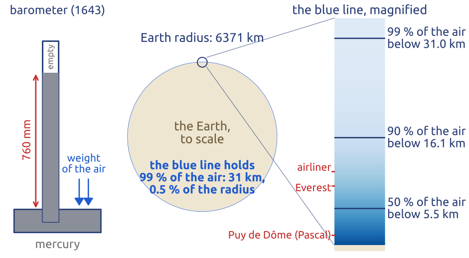
• Torricelli: the air has weight: it holds up 760 mm of mercury (the barometer)
• Pascal: on the Puy de Dôme the mercury stood about 8.5 cm lower (Périer’s climb, 1648): less air above
• Pressure is the weight of the air above, per unit area: the air is a thin skin

\[\frac{\partial p}{\partial z} = -\rho g\]

\(p\): pressure; \(z\): height; \(\rho\): density of the air; \(g\): gravity, 9.81 m/s²

Pressure is the weight of the air above; the air is a thin skin, half of it below 5.5 km

(Pascal 1648; Vallis 2017, sec. 1.3.3; NOAA et al. 1976)

Ask first: how much does the air above one square metre weigh? (About 10 tonnes: 101 325 Pa / g.) Périer, Pascal’s brother-in-law, measured 26 pouces 3.5 lignes at the foot and 23 pouces 2 lignes at the top, about 85 mm less. The hydrostatic balance is the vertical equation of most models. Next: Boyle. How heavy is a cubic metre of air? It depends on its temperature.

Boyle (1662): the spring of the air

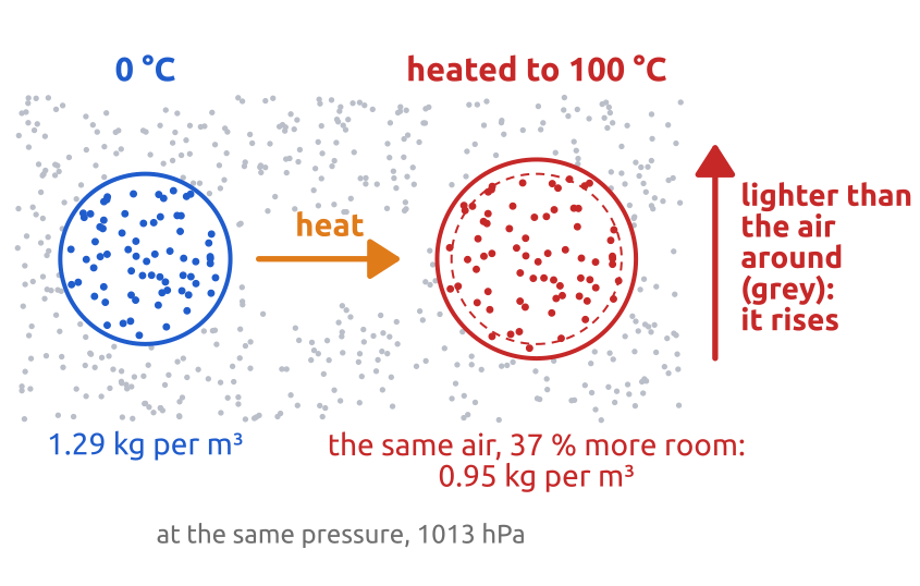
• Boyle’s law (1662): squeeze air and its pressure rises: at the same temperature, pressure × volume stays the same
• Heated air expands: warm air is lighter, and rises; Halley (1686): “rarified, and less ponderous”
• The exact law, at any temperature, came later: Charles’s and Gay-Lussac’s laws (around 1800)

\[p = \rho R T\]

\(p\): pressure; \(\rho\): density; \(T\): temperature (K); \(R = 287\) J/(kg K) for dry air

The gas law ties pressure, density and temperature: warm air is lighter, and rises

(Halley 1686, 165; Vallis 2017, sec. 1.4)

Ask first: heat a parcel of air from 0 to 100 °C at the same pressure: what happens to its size? (+37 %.) Boyle (1662) in his defence of “the spring and weight of the air”; Charles (1787), Gay-Lussac (1802). Halley’s words: Phil. Trans. 1686, p. 165 (original spelling “rarified”). R = 287 J/(kg K) for dry air. Heat and the first law: Carnot and Clausius, later today. Next: Halley (1686). Where is the air heated most? The Sun and the tropics.

Halley (1686): the Sun drives the winds

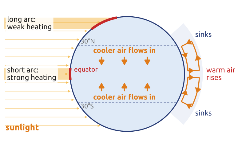
• Heated air rises, cooler air flows in

The Halley of the comet, back every 75–76 years.

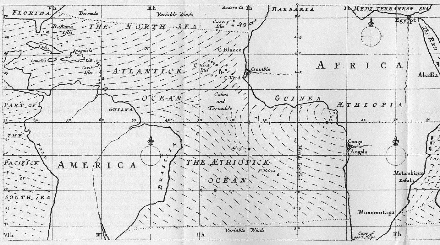
Halley’s map of the trade winds (Atlantic part).

Halley (1686), Philosophical Transactions; scan: Princeton University Library

• But the trade winds blow westward: why?
  • Halley: the Sun’s daily westward motion?

Dynamics: the tropics gain heat, the poles lose it: winds and currents carry it poleward

(Halley 1686, 165–67; Lorenz 1983, 731) · Map: commons.wikimedia.org: Edmond Halley’s map of the trade winds, 1686

Same beam: short arc at the equator, long arc near the pole: more heating in the tropics. Heating explains the inflow, not why it turns west. Halley: the Sun’s daily motion (wrong). Map: Atlantic part, sailors’ reports, 30N-30S. Comet: predicted its return for 1758.

Newton (1687): motion and gravity

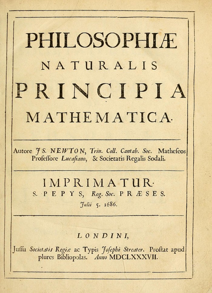
Principia, first edition, London, 1687. Public domain

• First law (inertia): a body keeps its velocity unless a force acts on it, seen from the fixed stars, not from the turning ground
• Second law: force = mass × acceleration; Euler (1755) will write it for every parcel of a fluid
• Gravitation: every mass attracts every other: the weight of the air, and the Moon’s pull on the ocean
• Halley persuaded Newton to write the Principia and paid for its printing

\[\underbrace{\mathbf{F} = m\,\mathbf{a}}_{\text{second law}} \qquad\qquad \underbrace{F = \frac{G\,m_1 m_2}{r^2}}_{\text{universal gravitation}}\]

\(\mathbf{F}\): force; \(m\): mass; \(\mathbf{a}\): acceleration; \(G\): gravitational constant; \(m_1, m_2\): masses at distance \(r\)

Halley’s question again: with no east–west push, air moving towards the equator keeps its motion in space, while the ground under it turns faster. What wind does it feel?

Newton’s laws: the physics under every model, and the key to Halley’s question

(Newton 1687) · Title page: commons.wikimedia.org: Newton’s Principia title page · Book: archive.org: Principia (1687)

Ask first: air leaves the tropics towards the equator; nothing pushes it east or west. Does it keep its speed over the ground, or its motion in space? Inertia holds in a frame that does not turn: the Earth’s surface turns (Coriolis, later today). Next: Hadley (1735). The answer to Halley’s question.

Hadley (1735): rotation turns the winds

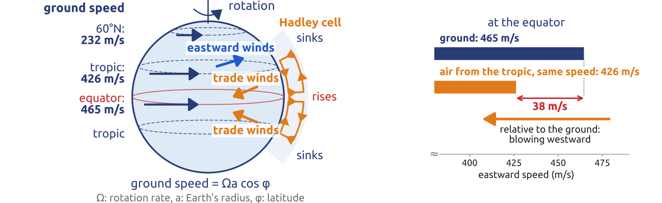
• Air moving towards the equator lags behind the ground: a wind blowing westward, the trade winds

• Air moving towards the poles runs ahead of the ground: a wind blowing eastward

• But 38 m/s is a storm: why?
  • Hadley: surface friction

The Earth’s rotation, not the Sun’s motion, “turns” the winds

(Hadley 1735; Persson 2006)

Ground: 465 m/s at the equator, 426 at the tropic (Hadley: “1000 to 917”). Air from the tropic lags 38 m/s: NE and SE trades. Returning high up, it runs ahead: an eastward wind. Hadley: 38 m/s beats “the greatest Storm”, so surface friction. Real trades: 5-10 m/s. Words: we say where the wind goes (eastward, westward); the usual names (easterly, westerly) say where it comes from: notes.

Angular momentum

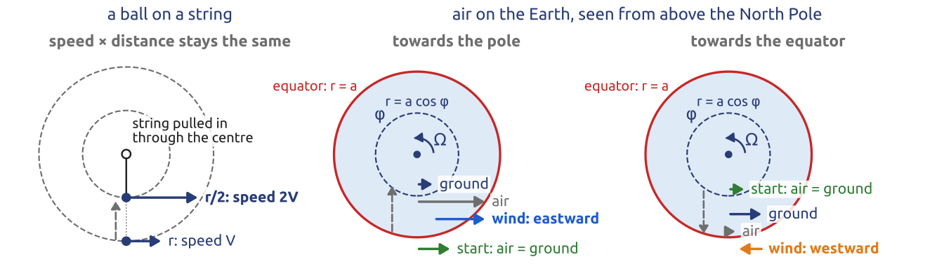
What it means: per unit mass, \(m = r\,V\): distance \(r\) to the axis × speed \(V\) around it. A pull towards the axis does not change it.

On the Earth (radius \(a\), rotation rate \(\Omega\), latitude \(\varphi\)): \(r = a\cos\varphi\), \(\;V\) = ground \(\Omega a\cos\varphi\) + wind \(u\) (westward if \(u<0\)): \(m = (\Omega a\cos\varphi + u)\,a\cos\varphi\)

Conservation of angular momentum, following the moving air: with no east–west push, \(Dm/Dt = 0\).

Towards a pole the air runs ahead of the ground, towards the equator it lags behind

(Persson 2006, 32; Vallis 2017, sec. 14.2)

Ball: the pull points to the axis, so speed x distance is kept (a skater). Earth: the same both ways; the wind is the air’s speed in space minus the ground’s. Hadley kept the speed instead: about half the effect.

In class: Hadley and angular momentum

Exercise 1 — Hadley’s argument and angular momentum. Air at rest over the equator rises and moves towards the pole, high up. What is its wind \(u\) at latitude \(\varphi\) if it keeps (a) its eastward speed in space \(V\), as Hadley (1735) assumed? (b) its angular momentum \(m\)? Compute \(u\) at \(10^\circ\), \(20^\circ\) and \(30^\circ\) and compare with the observed subtropical jet, 30–40 m/s. What could slow the air down?

\(u\) (m/s)	\(10^\circ\)	\(20^\circ\)	\(30^\circ\)
(a) keeping its speed in space (Hadley)
(b) keeping its angular momentum
observed (subtropical jet)			30–40

\(\Omega = 7.29\times10^{-5}\,\mathrm{s^{-1}}\), \(\;a = 6371\) km.

(c) To hand in: the other way round. Air at rest at \(30^\circ\) moves towards the equator, near the ground. Compute \(u\) at \(20^\circ\), \(10^\circ\) and \(0^\circ\) with (a) and (b), and compare with the trade winds, blowing westward at 5–10 m/s. What slows the air down here?

In notebook 01 (exercise 1.1): open in Colab · download

(Persson 2006, 32, 37; Vallis 2017, sec. 14.2)

Answers: (a) u = Ωa(1 − cos φ): 7, 28, 62 m/s. (b) u = Ωa sin²φ / cos φ: 14, 58, 134 m/s, about twice (a). Both too strong: aloft friction is weak; the eddies slow the air (lecture notes). (c) From 30°: Hadley −34, −55, −62; angular momentum −66, −104, −116 m/s: westward winds, slowed by surface friction.

Newton’s tide and the real ocean

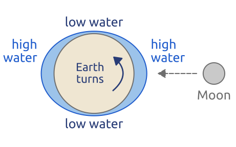
Newton (1687), the equilibrium tide: high water under the Moon, twice a day; M2 amplitude about 25 cm at the equator, less towards the poles.

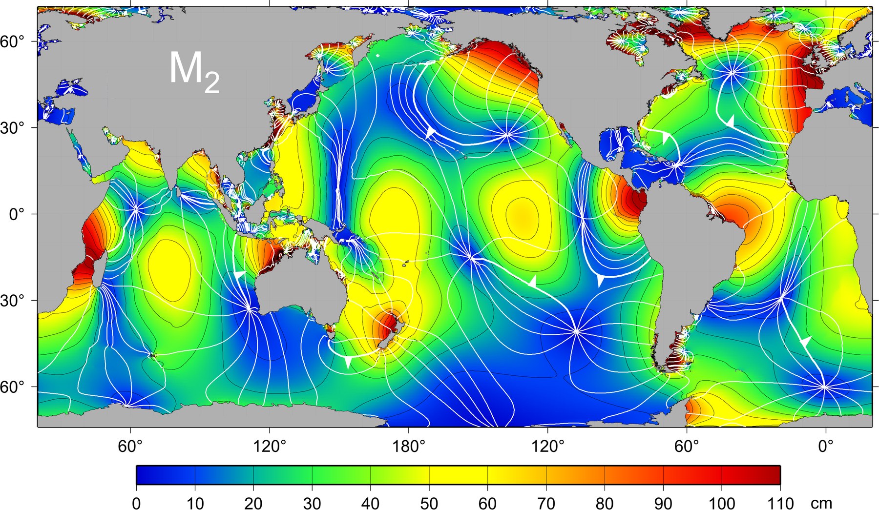
Observed: principal lunar semidiurnal tide (M2)

R. Ray, NASA Goddard Space Flight Center, from TOPEX/Poseidon satellite data

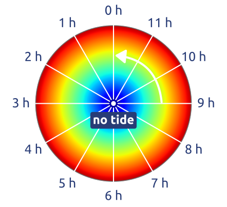
How to read it: colours, amplitude; white lines, high water at the same time, one hour apart. It turns around a point with no tide, the amphidromic point.

But: high water hours late, tides several times larger, points with no tide: the ocean moves as a fluid.

The Moon sets the rhythm; the ocean sets the size and the timing of the tide

(Hendershott 1981) · Map: commons.wikimedia.org: M2_Tidal_constituent.tif

Newton: M2 amplitude 24 cm at the equator, 6 cm at 60N (cos^2 lat); no tide only at the poles. Map: up to 1 m in the open ocean, largest at high latitudes; amphidromes; Fundy 15 m range. Map: find a point where the white lines meet (blue): no tide there. Question: why does the ocean not follow the Moon? Next slide.

Euler (1755): the equations of a fluid

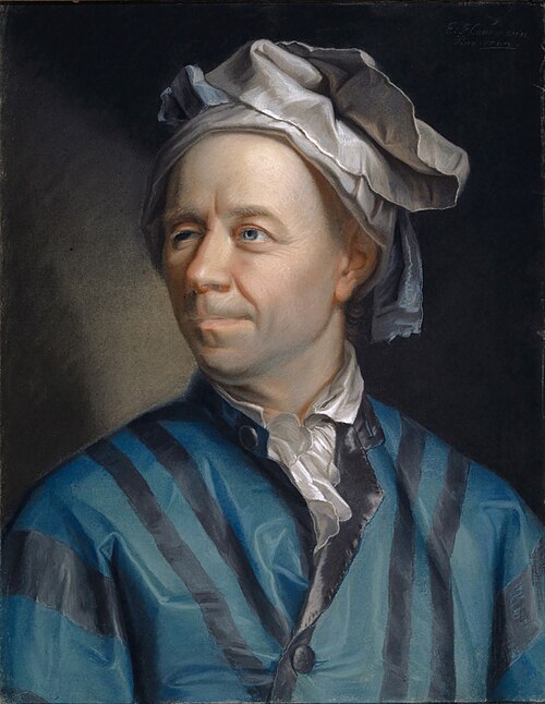
Leonhard Euler (1707–1783), by J. E. Handmann (1753). Public domain

• The fluid as a continuum: a velocity, a pressure and a density at every point
• Newton’s second law for every small parcel: mass × acceleration = pressure force + weight
• Mass is kept: what flows out of a small box empties it

\[\frac{D\mathbf{u}}{Dt} = -\frac{1}{\rho}\nabla p - \nabla\Phi, \qquad \underbrace{\frac{\partial\rho}{\partial t} + \nabla\cdot(\rho\mathbf{u}) = 0}_{\text{continuity equation}}\]

\(\mathbf{u}\): velocity; \(D/Dt\): change following a parcel; \(p\): pressure; \(\rho\): density; \(\Phi\): geopotential (gravity)

Newton’s laws for every parcel of a fluid: the base of every weather and ocean model

(Euler 1757; Vallis 2017; Chorin and Marsden 1993, sec. 1.1) · Portrait: commons.wikimedia.org: Leonhard Euler

Ask first: what forces act on a small cube of air? D/Dt: the change following the parcel (lecture 2). Phi: the geopotential (gravity). Laplace’s tidal equations (1776) came from Euler’s equations for a thin layer. Euler’s fluid has no friction: a body moving through it feels no drag (d’Alembert’s paradox, 1752): Navier and Stokes, later. Next: Laplace (1776). How does the ocean answer the Moon? These equations for a thin ocean on a rotating Earth.

Laplace (1776): the tides of a rotating ocean

• The ocean responds: tides are waves on a rotating Earth
• Too slow to follow the Moon: the point under the Moon moves at ~450 m/s, a tidal wave at \(\sqrt{gH} \approx 200\) m/s

\[\begin{aligned} \frac{\partial \mathbf{u}}{\partial t} + f\,\mathbf{k}\times\mathbf{u} &= -g\nabla(\eta - \eta_{eq})\\ \frac{\partial \eta}{\partial t} + \nabla\cdot(H\mathbf{u}) &= 0 \end{aligned}\]

\(\eta\): sea level; \(\mathbf{u}\): current; \(H\): depth; \(f = 2\Omega\sin\varphi\): the rotation; \(\eta_{eq}\): Newton’s tide (the forcing)

The linear shallow water equations.

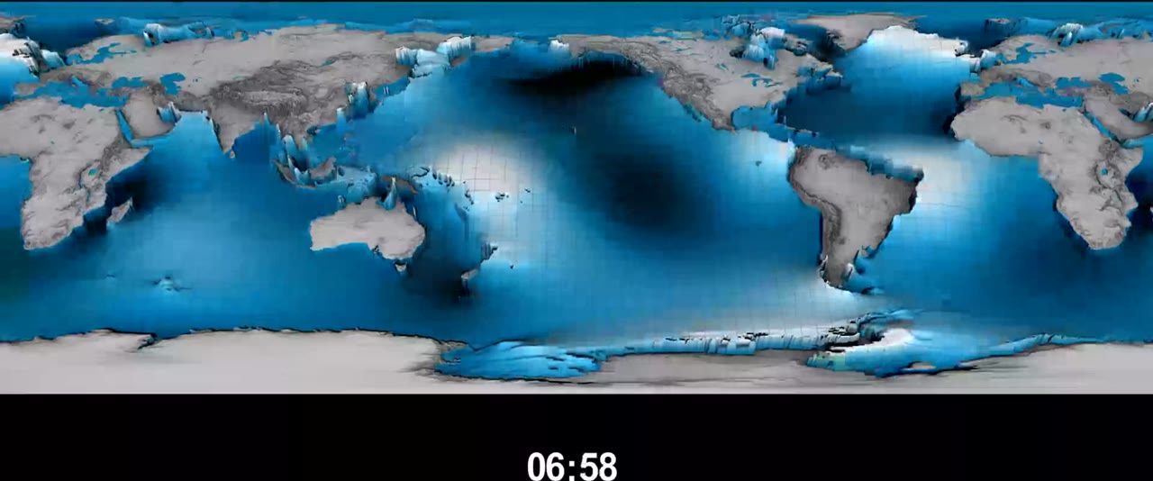
The global tide (mostly M2) over one day: high water turns around the amphidromic points.

NASA Goddard Scientific Visualization Studio (R. Ray, G. Shirah)

The tides are not a static bulge: they are waves in a rotating ocean

(Hendershott 1981) · Animation: svs.gsfc.nasa.gov/4821

Laplace’s equations: the shallow water equations (lecture 3), with the rotation term 60 years before Coriolis. Today solved on computers and checked against satellites, as in this animation.

Navier (1822), Stokes (1845): friction

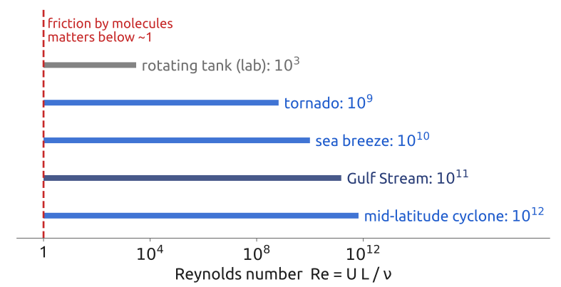
• Euler’s fluid has no friction. Navier, Stokes: add the friction between layers of fluid (the viscosity \(\nu\)): the Navier–Stokes equations
• How much it matters: the Reynolds number \(Re = UL/\nu\) (Reynolds, 1883)
• Winds and currents: \(Re \sim 10^{8}\)–\(10^{12}\): molecular friction is negligible, but the flow is turbulent, and eddies mix strongly

\[\frac{D\mathbf{u}}{Dt} = -\frac{1}{\rho}\nabla p - \nabla\Phi + \nu\nabla^2\mathbf{u}\]

\(\nu\): kinematic viscosity (air \(1.5\times10^{-5}\), water \(10^{-6}\) m²/s); \(\mathbf{u}\), \(p\), \(\rho\), \(\Phi\): as in Euler

Molecular friction is negligible at large scales; turbulence is not, and must be modelled

(Navier 1827; Stokes 1845; Reynolds 1883; Cushman-Roisin and Beckers 2011, sec. 4.5)

Ask first: honey, water, air: which flow is “more viscous” at the scale of a cyclone? nu: 1.5e-5 m^2/s for air, 1e-6 for water. Computing every eddy, down to millimetres, needs about 5e27 points (the atmosphere, 5e18 m^3, on a 1-mm grid): models compute the large scales and model the rest. Turbulent friction near the ground: the Ekman layer; in models: parameterizations. Next: Carnot, Clausius. The air is also heated and cooled: what does heat do to moving air?

Carnot (1824), Clausius (1850): heat and work

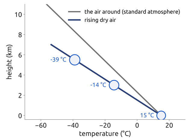
• Carnot (1824): heat engines. Clausius (1850): heat and work, and the first law of thermodynamics, the conservation of energy: heating a parcel raises its temperature, or makes it expand
• Rising air expands and cools, faster than the air around it usually does: cold mountain tops, clouds in rising air

\[c_p\frac{DT}{Dt} - \frac{1}{\rho}\frac{Dp}{Dt} = Q\]

\(T\): temperature; \(p\): pressure; \(\rho\): density; \(c_p = 1004\) J/(kg K): specific heat; \(Q\): heating per unit mass

Heat and motion are tied: rising air expands and cools

(Clausius 1850; Wallace and Hobbs 2006, ch. 3)

Ask first: air rises 1 km up a mountain without exchanging heat: warmer or colder? How much colder (g/c_p, 9.8 K/km dry) is computed in lecture 3, exercise 1. The observed mean, 6.5 K/km, is smaller: condensation (latent heat) and radiation. Rising air colder than its surroundings sinks back: the atmosphere is stable (lecture 4). Next: Coriolis (1835). We measure all this on a turning Earth: what does the rotation add?

Coriolis (1835): a planar rotating frame (disk)

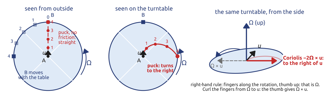
• Newton’s laws hold in a frame that does not turn; we measure winds on the turning Earth
• Seen from the Earth: the Coriolis force \(-2\boldsymbol{\Omega}\times\mathbf{u}\)

Laplace (1776) had it for the tides; Coriolis made it general.

\[\frac{D\mathbf{u}}{Dt} + 2\boldsymbol{\Omega}\times\mathbf{u} = -\frac{1}{\rho}\nabla p - \nabla\Phi\]

\(\boldsymbol{\Omega}\): Earth’s rotation; \(\mathbf{u}\): velocity on the Earth; \(p\), \(\rho\), \(\Phi\): pressure, density, geopotential

The Coriolis force turns moving air and water; it never speeds them up

(Coriolis 1835; Persson 1998)

Puck pushed from A towards B, sliding without friction (air hockey): from outside it goes straight while B moves away; on the table it turns right. Same table from the side: Omega up, u north, Omega x u west, force east: to the right. Coriolis worked on water wheels, not weather; meteorology got the term from Laplace’s tides via Foucault and Ferrel. Persson (1998): it would just have been named after Foucault or Ferrel. Name: “deflective force” in the 1800s, “Coriolis force” only after 1900; the letter f may honour Foucault or Ferrel (Persson’s guess).

Foucault (1851): the local rotation

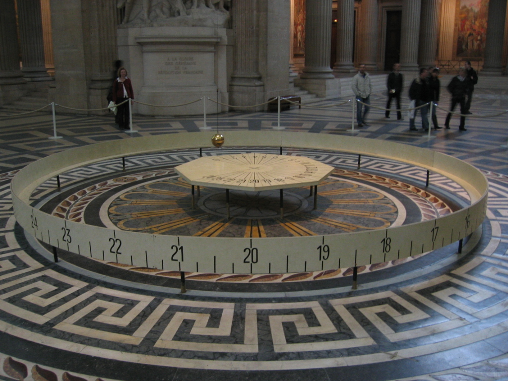
The pendulum in the Panthéon (today’s copy). Arnaud 25, Wikimedia Commons · ▶ videos (online): in Italian, short

1. The bob swings in a fixed plane: nothing pushes it sideways
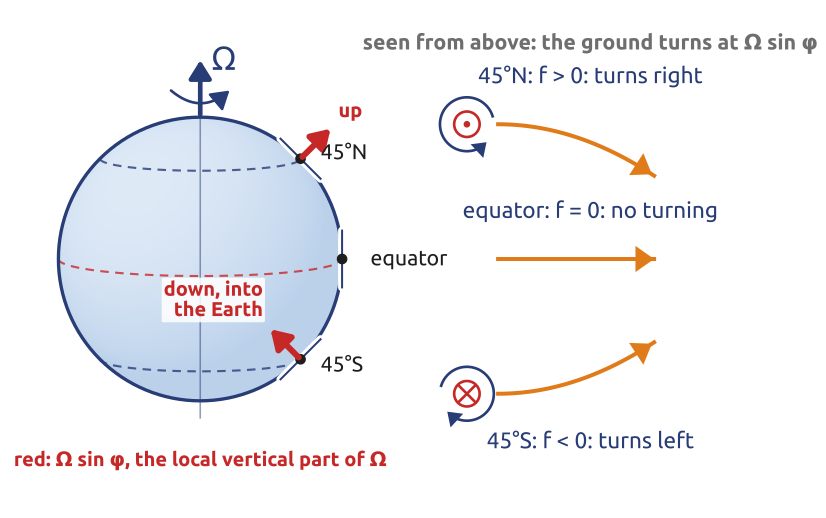
2. Under it, the floor turns with the Earth itself, at \(\Omega\sin\varphi\) (Paris: \(\varphi = 48.9^\circ\)N)
3. Seen from the floor, the swing turns clockwise: once in \(24\,\mathrm{h}/\sin 48.9^\circ \approx 32\) h (Milan: 34 h)

The Coriolis parameter \(f = 2\Omega\sin\varphi\) turns motion right in the northern hemisphere, left in the southern

(Foucault 1851; Persson 1998) · Photo: commons.wikimedia.org: Pendule de Foucault.jpg · Videos: youtu.be/oyH5438wBcU, youtu.be/59phxpjaefA

Panthéon, 1851: 67 m wire, 28 kg bob. Gravity and the wire’s pull lie in the plane of swing. No turntable: the floor is the Earth. Milan: 34 h. At the equator f = 0: no turning. Videos need internet: TuttoGreen 2025 (Italian, at the Panthéon), B. Florescu 2012 (short). The pendulum feels only the local vertical part of the rotation, Omega sin(lat): it measures f/2. A free parcel turns twice as fast: inertial loops every 12 h / sin(lat), 17 h at Milan, drawn by drifting buoys in the ocean.

The Coriolis force in components

Horizontal motion feels only the part of \(\boldsymbol{\Omega}\) along the local vertical \(\mathbf{k}\):

\[\begin{aligned} \frac{d\mathbf{u}}{dt} &= -2\boldsymbol{\Omega}\times\mathbf{u} \;\to\; -f\,\mathbf{k}\times\mathbf{u}\\[2pt] \mathbf{k}\times\mathbf{u} = (-v,\, u) \;&\Rightarrow\; \frac{du}{dt} = f\,v, \quad \frac{dv}{dt} = -f\,u \end{aligned}\]

\(f = 2\Omega\sin\varphi\): the Coriolis parameter, twice the local rotation rate

• \(u\) east, \(v\) north. Moving east (\(u>0\)): \(v\) decreases, it turns south; then \(u\) decreases: it keeps turning right
• The speed \(U = |\mathbf{u}|\) does not change: a circle of radius \(U/f\), once every \(2\pi/f\): 17 h at Milan (pendulum: 34 h)

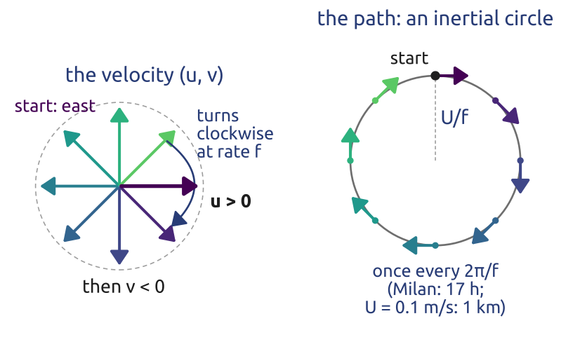
\(u\) feeds \(v\) and \(v\) feeds \(u\): moving water and air turn in circles, the inertial oscillations

(Cushman-Roisin and Beckers 2011, sec. 2.3; Persson 1998, 1377)

Only Omega sin(lat) acts on horizontal motion; the Omega cos(lat) part gives small vertical forces (dropped for thin layers, later). -f k x u = (f v, -f u). Solution: u turns clockwise at rate f. Twice the pendulum’s rate: the swing shows one half, the ground turning under the moving air (Omega sin lat); the other half: the parcel reaches ground moving at another speed, which is the half Hadley kept (lecture 2, the two terms of 2 Omega x u). Ferrel (next) adds the pressure force: the balance of the two is the geostrophic wind.

Ferrel (1856–58): wind along the isobars

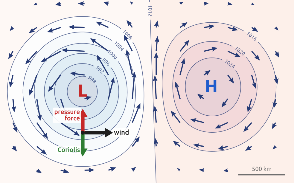
\[f\,\mathbf{k}\times\mathbf{u}_g = -\frac{1}{\rho}\nabla p \quad\Longleftrightarrow\quad \mathbf{u}_g = \frac{1}{\rho f}\,\mathbf{k}\times\nabla p\]

\(\mathbf{u}_g\): geostrophic wind; \(f = 2\Omega\sin\varphi\); \(\mathbf{k}\): vertical; \(p\), \(\rho\): pressure, density

The previous slide, plus the pressure force:

\[\begin{aligned} \frac{du}{dt} &= f\,v - \frac{1}{\rho}\frac{\partial p}{\partial x}, & \frac{dv}{dt} &= -f\,u - \frac{1}{\rho}\frac{\partial p}{\partial y}\\[4pt] u_g &= -\frac{1}{\rho f}\frac{\partial p}{\partial y}, & v_g &= \frac{1}{\rho f}\frac{\partial p}{\partial x} \end{aligned}\]

Second line: the forces balance: the geostrophic wind

• Not from high to low pressure: along the isobars, anticlockwise round a low (northern hemisphere)
• Buys Ballot’s law (1857), from weather maps: in the northern hemisphere, wind at your back, low pressure on your left
• But: a sea breeze blows from high to low. When does the rotation win?

Large, slow winds blow along the isobars: the pressure force and the Coriolis force balance

(Ferrel 1858; Persson 1998, 1376; Vallis 2017, sec. 2.8.2)

South of the low: wind east, pressure force north, Coriolis south: balanced, so no turning. Faster where the isobars are closer. Near the ground friction slows the wind: it crosses the isobars towards the low. Small, fast motions: rotation too slow to matter (exercise 2).

In class: does it feel the Earth’s rotation?

Exercise 2 — Does it feel the Earth’s rotation? For each phenomenon, estimate a typical speed \(U\) and size \(L\), then the Rossby number \(Ro = U/(fL)\), with \(f = 2\Omega\sin\varphi\) and \(\Omega \approx 7.29\times10^{-5}\,\mathrm{s^{-1}}\). Start with \(f\) at Milan (\(\varphi = 45.5^\circ\) N). Rotation matters when \(Ro \lesssim 1\).

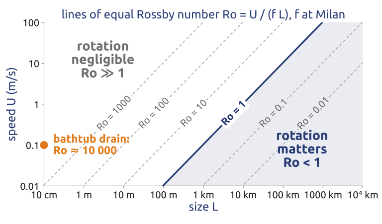
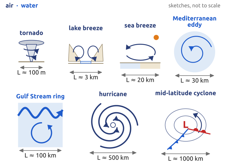
To hand in: nearer the equator. Redo it for a place of your choice between the equator and \(15^\circ\) (north or south). At what latitude does a mid-latitude cyclone (\(U = 10\) m/s, \(L = 1000\) km) reach \(Ro = 1\)?

In notebook 01 (exercise 2.1): open in Colab · download

(Vallis 2017, sec. 2.8.1; Cushman-Roisin and Beckers 2011, sec. 4.5)

f at Milan = 1.04e-4 1/s. Typical U, L and Ro: sea breeze 5 m/s, 20 km, 2.4 · lake breeze 3 m/s, 3 km, 10 · tornado 50 m/s, 100 m, 5000 · hurricane 40 m/s, 500 km, 0.8 · cyclone 10 m/s, 1000 km, 0.1 · Gulf Stream ring 1 m/s, 100 km, 0.1 · Mediterranean eddy 0.2 m/s, 30 km, 0.06. Bathtub: Ro 10^4, the Earth does not choose the way the water turns. Ocean: slower, smaller. Hand-in: |f| = 2 Omega sin(lat), smaller near the equator, Ro larger. Cyclone: Ro = 1 where sin(lat) = U/(2 Omega L) = 0.07, about 4 degrees: no geostrophy (and no hurricanes) near the equator.

Observing the ocean, 1769–1876

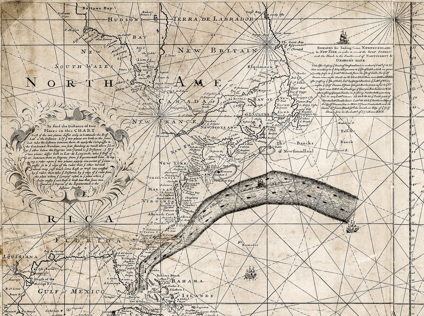
Franklin–Folger chart of the Gulf Stream, London, 1769. Library of Congress

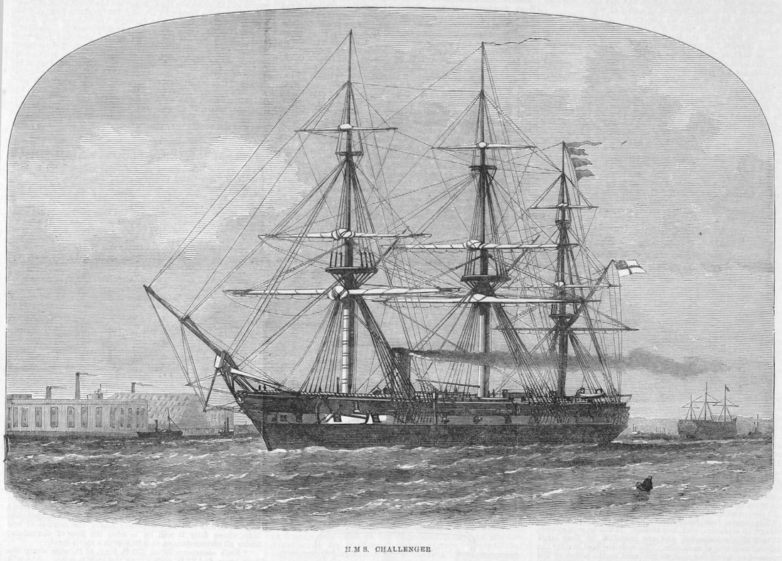
HMS Challenger. The Illustrated London News, 1872

• Franklin, postmaster: mail ships from England took two weeks longer than merchant ships. Captain Folger: they sailed against the Gulf Stream
• Maury (US Navy, 1847–1855): charts from ships’ logs
• Challenger (1872–1876): the first survey of the deep ocean
• But: what drives them: density differences or the wind?

Ships mapped the currents long before any theory could explain them

(Franklin 1786, 314–15; Stewart 2008, sec. 2.3; Warren 1981, sec. 1.2) · Chart: Commons · Engraving: Commons

Franklin’s own account: the mail packets Falmouth-New York took two weeks longer than merchant ships; Folger: Nantucket captains knew the stream. Maury traded charts for logbooks. Challenger: depths and temperatures in every ocean. Carpenter and Croll argued in the 1870s; both were partly right: density (Bjerknes, next) and wind (Ekman, after).

Kelvin (1869): circulation, the spin of a fluid

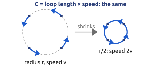
Kelvin (1869): with no friction, the circulation of a loop moving with the fluid is kept, at constant density and in any barotropic fluid (density set by pressure alone; Silberstein, 1896)

\[C = \oint \mathbf{u}\cdot d\mathbf{l}, \qquad \frac{DC}{Dt} = 0\]

\(C\): circulation (spin) of a loop; \(d\mathbf{l}\): piece of the loop

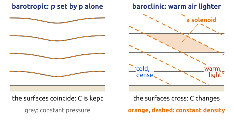
But: in a barotropic fluid at rest, nothing ever starts to turn. How do winds and currents start?

Without friction, in a barotropic fluid, spin is kept: a shrinking loop spins faster

(Thomson 1869; Thorpe et al. 2003)

C = 2 pi r v: the ball on a string of the angular momentum slide, for a whole loop. Kelvin: constant density (read 1867); the barotropic form is how Vallis and Holton state it. Silberstein 1896: the barotropic case; a fluid at rest starts to turn only where the surfaces cross. Barotropic: temperature uniform on each pressure surface; baroclinic: fronts, sea breezes, the pole-to-equator contrast. The rotating Earth (zeta + f): Rossby.

Bjerknes (1898): how winds and currents start

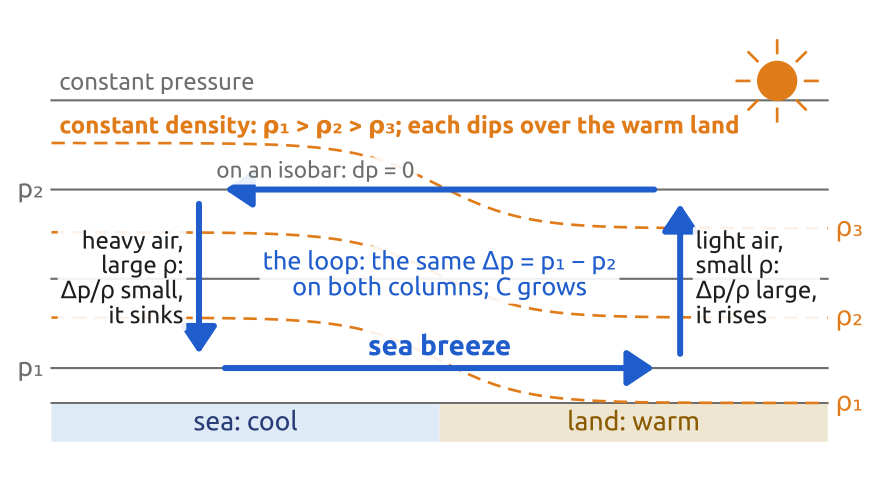
Silberstein (1896) found it first: a fluid at rest starts to turn if, and only if, its surfaces of constant pressure and density cross (baroclinic). Bjerknes applied it to air and sea.

1. The Sun warms the land more than the sea: at the same pressure, warm air is lighter
2. Both columns span the same \(\Delta p = p_1 - p_2\); per kilogram the push is \(\Delta p/\rho\): larger for the light air
3. The light air rises, the heavy air sinks: a breeze from the sea

\[\begin{aligned}\frac{DC}{Dt} &= -\oint\frac{dp}{\rho}\\ &= \Delta p\left(\frac{1}{\rho_{\mathrm{land}}} - \frac{1}{\rho_{\mathrm{sea}}}\right) > 0\end{aligned}\]

\(C\): circulation around the loop; \(p\): pressure; \(\rho\): density; \(\Delta p = p_1 - p_2\)

Uneven heating makes density differences, and density differences make winds and currents

(Bjerknes 1898; Thorpe et al. 2003; Vallis 2017, sec. 4.3)

Silberstein (1896) had it first. Bjerknes: breezes, monsoons, trade winds, cyclones, a chimney, and the oceans (warm or fresh water is lighter: Carpenter’s side). His Fig. 9 is this sea breeze. Bjerknes (1902) added the Earth’s rotation. Next: Teisserenc de Bort and Assmann (1902), with balloons. What does the air look like above our heads?

Teisserenc de Bort, Assmann (1902): layers

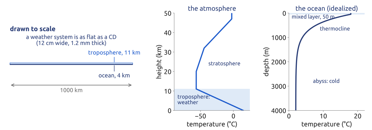
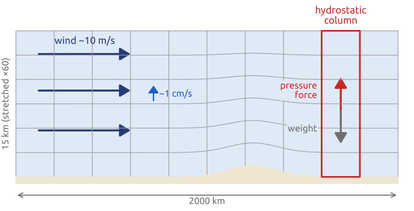
Thin: 10 km of air, 4 km of water, systems 1000 km wide: motions are mostly horizontal

Layered: with balloons, Teisserenc de Bort and Assmann (1902) found that the air stops cooling above ~11 km: the troposphere under the stratosphere. Ocean: warm water over a cold abyss

Hydrostatic balance: in each column, the pressure is the weight above.

The atmosphere and the ocean are thin, layered, nearly hydrostatic shells on a rotating sphere

(Vallis 2017, sec. 2.7 and Ch. 15, endnote 7 (p. 583); Cushman-Roisin and Beckers 2011, sec. 4.3)

Ask first: if the Earth were a globe 30 cm across, how thick would the troposphere be? (A quarter of a millimetre.) Aspect ratio H/L about 10^-2 for weather systems, 10^-3 for the ocean basins. Next: Bjerknes (1904). Can we compute tomorrow’s weather?

Bjerknes (1904): an initial-value problem

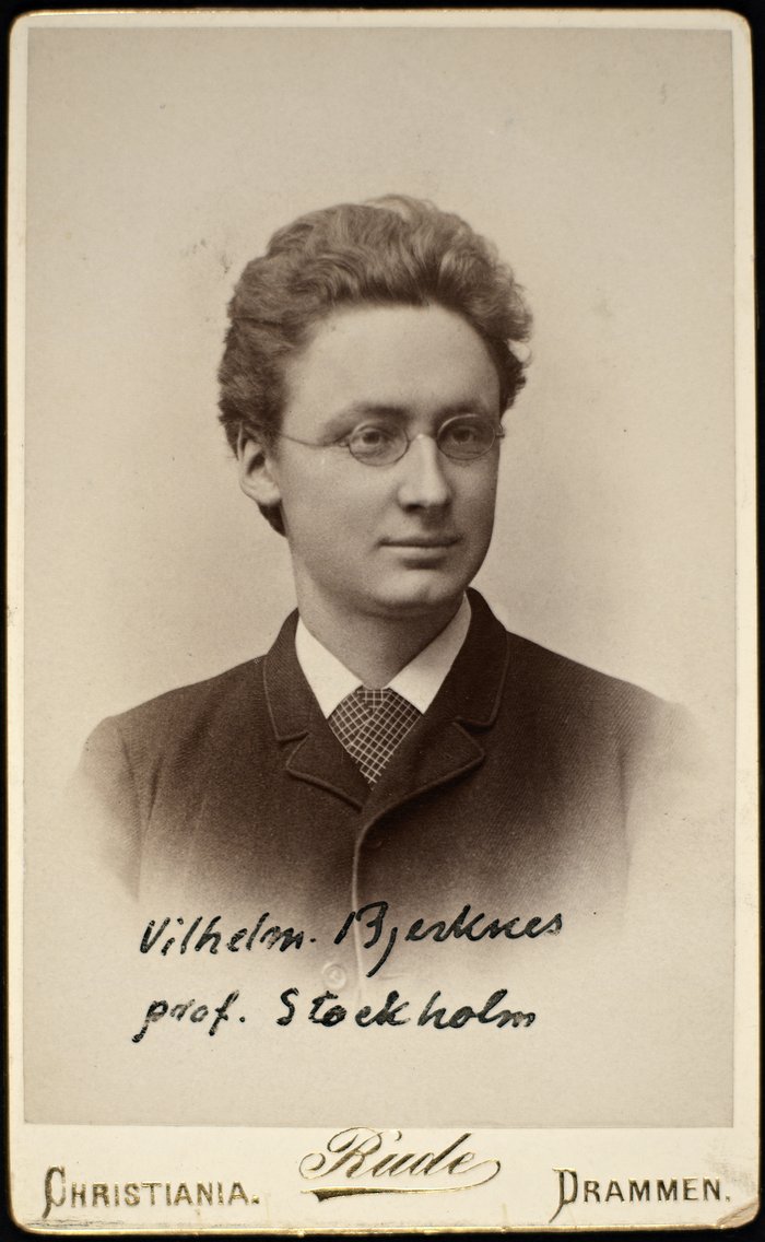
Vilhelm Bjerknes (1862–1951). Nasjonalbiblioteket, CC BY 2.0

A rational forecast needs: “1. […] the state of the atmosphere at a given time. 2. […] the laws according to which one state of the atmosphere develops from another.”

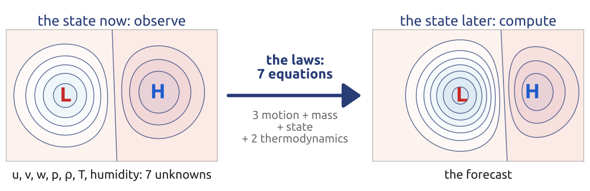
But: “There can be no question of a strictly analytical integration”: no formula solves the equations (not even three bodies under gravity). Bjerknes: step the maps forward hour by hour, graphically.

A forecast is an initial-value problem: observe the state now, integrate the laws forward

(Bjerknes 1904; Lynch 2008b) · Photo: commons.wikimedia.org: Portrett av Vilhelm Bjerknes

Seven unknowns, seven equations; today the 7th is the water-vapour equation. Diagnosis, then prognosis. Even three bodies under Newton’s law cannot be solved exactly. Abbe (1901) said much the same in the US. Bergen school: fronts and air masses. Next: Richardson (1922), with numbers.

Ekman (1905): the wind-driven ocean

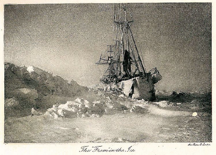
The Fram. Nansen (1897), Farthest North

Nansen (Fram, Arctic, 1893–96): the ice drifted 20–40° right of the wind

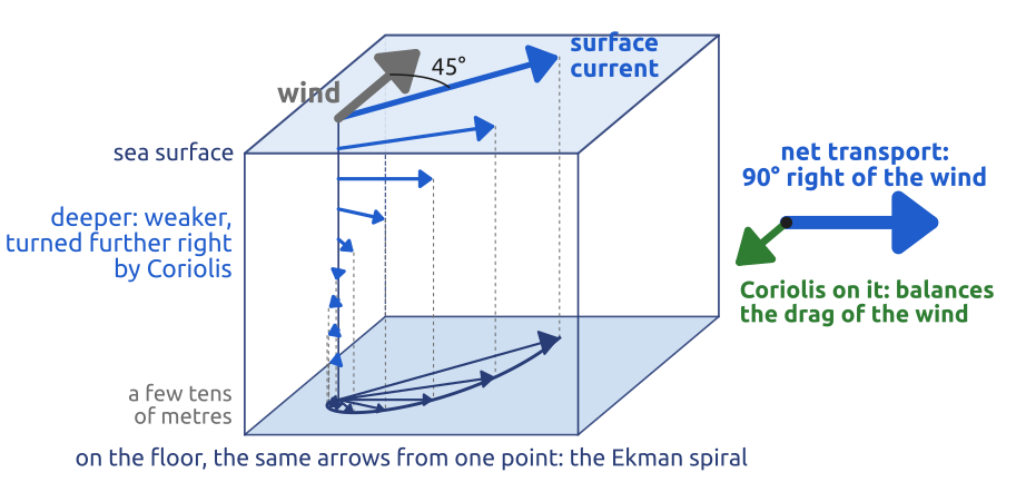
Ekman (1905): the layer moves \(90^\circ\) right of the wind (northern hemisphere). The ice moves with the surface water: \(45^\circ\) in Ekman’s model, less with real mixing: Nansen’s 20–40°

But: why is the Gulf Stream narrow, fast, and off America, not Europe?

\[\mathbf{M}_E = \frac{\boldsymbol{\tau}\times\mathbf{k}}{\rho_0 f}\]

\(\mathbf{M}_E\): volume transport per unit width (m²/s); \(\boldsymbol{\tau}\): wind stress; \(\rho_0\): water density; \(f = 2\Omega\sin\varphi\); \(\mathbf{k}\): vertical

Coriolis balances the drag of the wind: the wind-driven layer moves at right angles to the wind

(Ekman 1905; Stewart 2008, sec. 9.2; Munk 2002, 136) · Photo: commons.wikimedia.org: FMIB 32687 The Fram in the Ice

Ask first: the wind blows north over a still sea; which way does the water go? The wind side of Carpenter and Croll’s dispute. 1900: Nansen asked Bjerknes; his student Ekman solved it, it is said, that evening (Munk). Steady: forces on the layer cancel; Coriolis is the only sideways one, so the motion is 90° right. M_E: volume transport per unit width (Vallis’s M_E is the mass transport, times rho_0), tau: wind stress; no friction coefficient in it. Spiral derived in lecture 3. Answered by Stommel (1948), later today (gyres slide).

Richardson (1922): the laws, by numbers

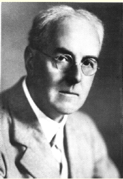
Lewis Fry Richardson (1881–1953). NOAA, public domain

\[\begin{aligned} &\text{momentum:} && \frac{D\mathbf{u}_h}{Dt} + f\,\mathbf{k}\times\mathbf{u}_h = -\frac{1}{\rho}\nabla_h p + \mathbf{F}\\[2pt] &\text{hydrostatic balance:} && \frac{\partial p}{\partial z} = -\rho g\\[2pt] &\text{continuity:} && \frac{D\rho}{Dt} + \rho\,\nabla\cdot\mathbf{u} = 0\\[2pt] &\text{first law, ideal gas:} && c_p\frac{DT}{Dt} - \frac{1}{\rho}\frac{Dp}{Dt} = Q, \qquad p = \rho R T \end{aligned}\]

\(\mathbf{u}_h\), \(\nabla_h\): horizontal wind and gradient; \(f = 2\Omega\sin\varphi\); \(\mathbf{F}\): friction; \(p\), \(\rho\), \(T\): pressure, density, temperature; \(Q\): heating; \(R\), \(c_p\): gas constant, specific heat

Bjerknes’ laws on a chequerboard of squares about 200 km wide: derivatives become finite differences, stepped forward in time

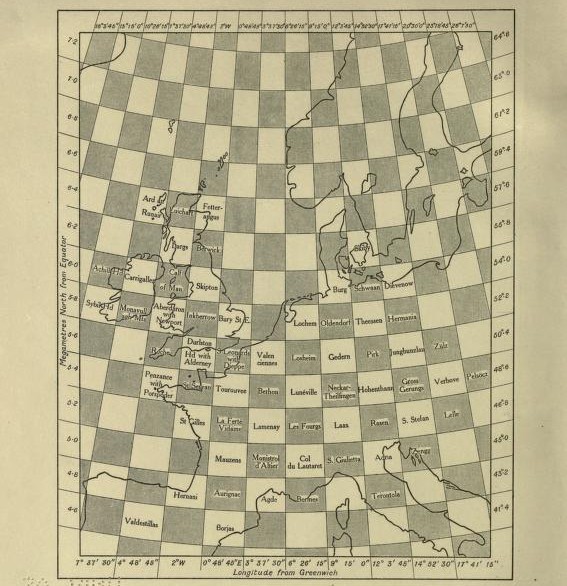
Richardson (1922), frontispiece: pressure and wind in alternate squares. Public domain

By hand: a forecast six hours ahead, computed on paper: about six weeks of computing, spread over some two years, while he drove an ambulance in France in the war

The first forecast by numbers: the laws on a grid, stepped forward in time

(Richardson 1922, 219; Lynch 1999, 61–68; Hunt 1998) · Portrait: commons.wikimedia.org: Lewis_Fry_Richardson.png · Grid: archive.org/details/weatherpredictio00richrich

Ask first: how long would a six-hour forecast for two points take by hand? Five layers, columns about 200 km apart; time step 3 h, a step-over (leapfrog) across 6 h (Lynch 1999). “On a heap of hay in a cold wet rest billet” (Hunt 1998). Equations: lecture 2; finite differences: lecture 5.

Richardson’s dream: the forecast factory

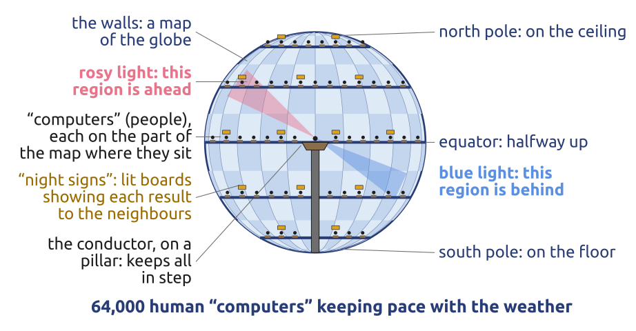
Sketch from Richardson’s own description (1922, p. 219) · ▶ the painting by Stephen Conlin (1986), online

The result: surface pressure rising 145 hPa in 6 hours; “observations show that the barometer was nearly steady”

Why: winds and pressures slightly out of balance set off fast gravity waves, which swamped the slow weather

The dream: 64,000 people in a hall, each computing one region, a conductor keeping them in step: “Perhaps some day in the dim future it will be possible to advance the computations faster than the weather advances […] But that is a dream.”

What he left: observe the state, put it on a grid, step the laws forward, faster than the weather

It failed badly, but it left the method of every operational forecast since

(Richardson 1922, vii, 187, 219; Lynch 2008b, secs. 1.2–1.3) · The factory: emetsoc.org: Richardson’s Fantastic Forecast Factory

Ask first: 145 hPa in 6 h: where can such an error come from? Lynch reran it: the same 145 hPa; from balanced data, under 1 hPa (lecture 3). The factory: an early massively parallel computer (Lynch 2008); 1950 did it with one machine (lecture 5). The Met Office’s new model, LFRic, is named after him (lectures 8, 9).

Rossby (1939): waves in the mid-latitude winds

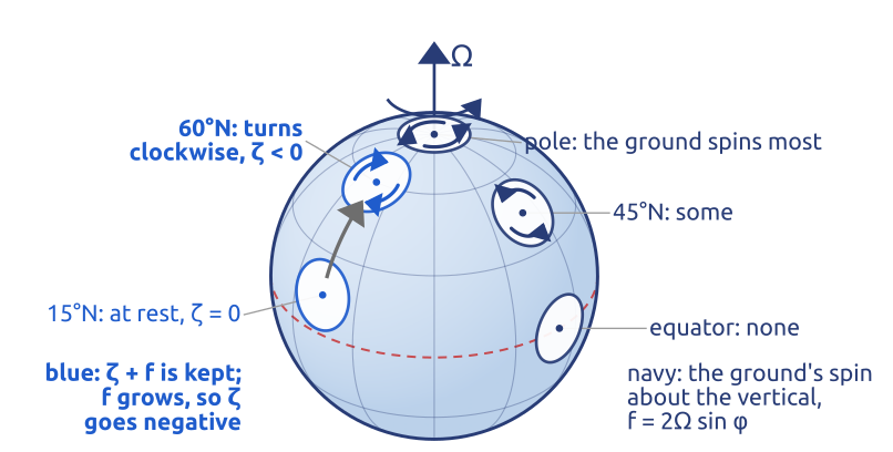
Vorticity \(\zeta = \partial_x v - \partial_y u\): the spin of a small column relative to the ground. A column keeps its total spin \(\zeta + f\): carried north, \(f\) grows, so \(\zeta < 0\): it turns clockwise seen from above. \(f\) grows northward in both hemispheres: the waves drift west in both

A catch: the wind carries them: cyclones still travel east

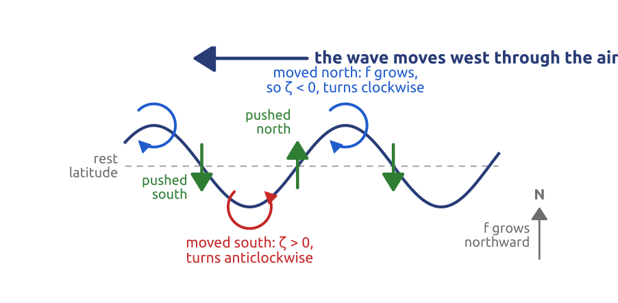
\[\frac{D}{Dt}(\zeta + f) = 0 \qquad \beta = \frac{df}{dy} > 0\] \[\underbrace{c}_{\substack{\text{wave speed}\\ \text{relative to the ground}}} = \underbrace{U}_{\text{wind}} - \underbrace{\frac{\beta}{k^2}}_{\substack{\text{drift west}\\ \text{through the air; } k = 2\pi/L}}\]

Because \(f\) grows to the north, the waves drift west, against the wind that carries them

(Rossby and collaborators 1939; Vallis 2016)

Ask first: a column carried north keeps zeta + f: which way does it turn? beta = 2 Omega cos(lat) / a = 1.6e-11 1/(m s) at 45 N. Against an eastward wind U the wave stands still when U = beta/k^2: wavelength 2 pi sqrt(U/beta), about 6000 km for 15 m/s: 4–5 waves round the Earth. Hough (1898) had found these waves in Laplace’s tidal equations. The catch, U = 15 m/s: L = 4000 km moves east at 8 m/s; 6000 km stands still; 10,000 km drifts west at 25 m/s.

Rossby waves on the jet: August 2002

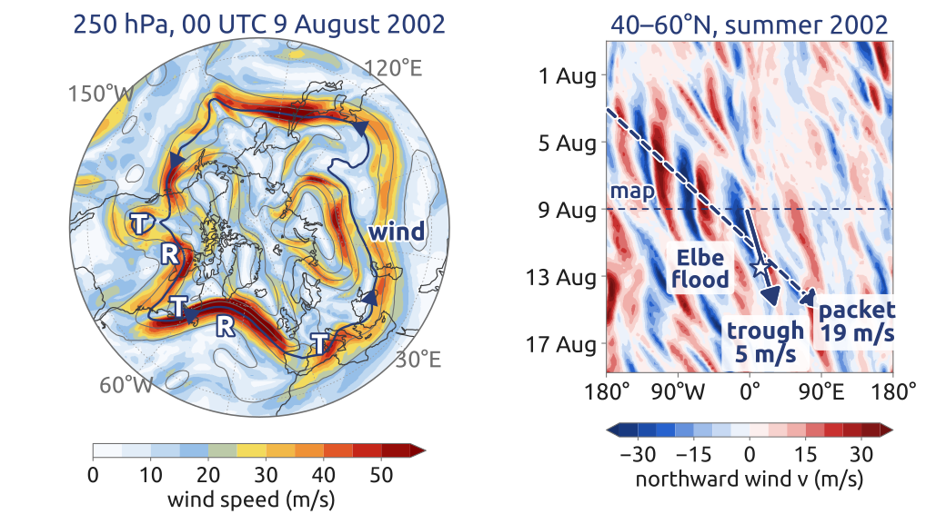
Left: 250 hPa, 00 UTC 9 Aug 2002; colours: wind speed; lines: geopotential height every 120 m (navy: 10,680 m). Right: northward wind \(v\) at 250 hPa, 40–60°N mean, every 6 h, longitude against time (a Hovmöller diagram); arrows: a trough, the packet; star: Elbe flood

ERA5 (Hersbach et al. 2020); contains modified Copernicus Climate Change Service information [2026]

Troughs (T) and ridges (R): the jet meanders around the hemisphere; the wind along it steers the cyclones. Right: air going north (red), south (blue)

Each trough moves east, about 5 m/s, slower than the wind (16 m/s): relative to the air it drifts west, 16 − 5 ≈ 11 m/s, Rossby’s \(\beta/k^2\)

The packet of large waves runs east faster, 19 m/s: from the Pacific (3 Aug) to Europe, where it came with the low whose rain flooded the Elbe (12–13 Aug)

On the jet, troughs crawl east, slower than the wind; the wave packet runs ahead

(Wirth et al. 2018, 1966–72; Hovmöller 1949; Ulbrich et al. 2003, 371) · Data: cds.climate.copernicus.eu: ERA5 hourly data on pressure levels

Ask first: on the right, which way do the stripes move, and which way does the band of strong colours move? Hovmöller (1949) drew such diagrams by hand (500 hPa geopotential height, winter 1945–46). Packet faster than the troughs, even than the wind: the group speed, U + β/k² (Rossby 1945). Elbe: the low formed over the Gulf of Genoa on 10 August; 312 mm in 24 h at Zinnwald; Dresden’s highest water since 1275 (Ulbrich et al. 2003). Next: a wave that does not move at all: summer 2026. Ocean (if asked): Rossby waves cross the Pacific westward, months near the equator, ~10 years at mid-latitudes; no strong eastward current carries them (Chelton and Schlax 1996).

Blocks: when a Rossby wave stands still

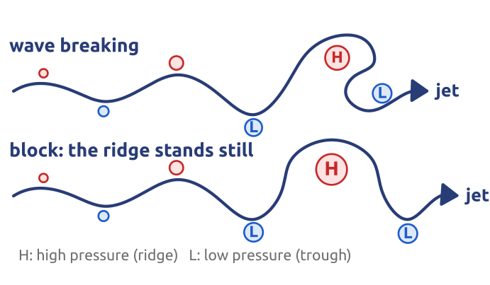
A Rossby wave on the jet can grow until it breaks (the crest overturns) or blocks: a large ridge stands still, a low on each side (an omega), and the jet goes around it

\[c = U - \frac{\beta}{k^2} = 0 \;\Longrightarrow\; L_s = 2\pi\sqrt{\frac{U}{\beta}}\]

\(c\): wave speed over the ground; \(U\): eastward wind; \(\beta = df/dy\); \(k = 2\pi/L\); \(L_s\): the wavelength that stands still

With \(U \approx 10\) m/s at 50°N: \(L_s \approx 5000\) km, the size of a block

Long Rossby waves can stand still against the wind: a large ridge that stalls is a block

(Holton 2004, sec. 7.7.1; Woollings et al. 2018)

Ask first: the wind carries a wave east, β makes it drift west: which waves stand still? β = 1.47e-11 1/(m s) at 50°N; U = 10 m/s gives L_s = 5200 km, about 5 waves round the latitude circle. Breaking: the wave overturns and mixes; blocking: it stalls. Both are nonlinear; only “can stand still” is linear. Next: the block of summer 2026.

Blocking over Europe: summer 2026

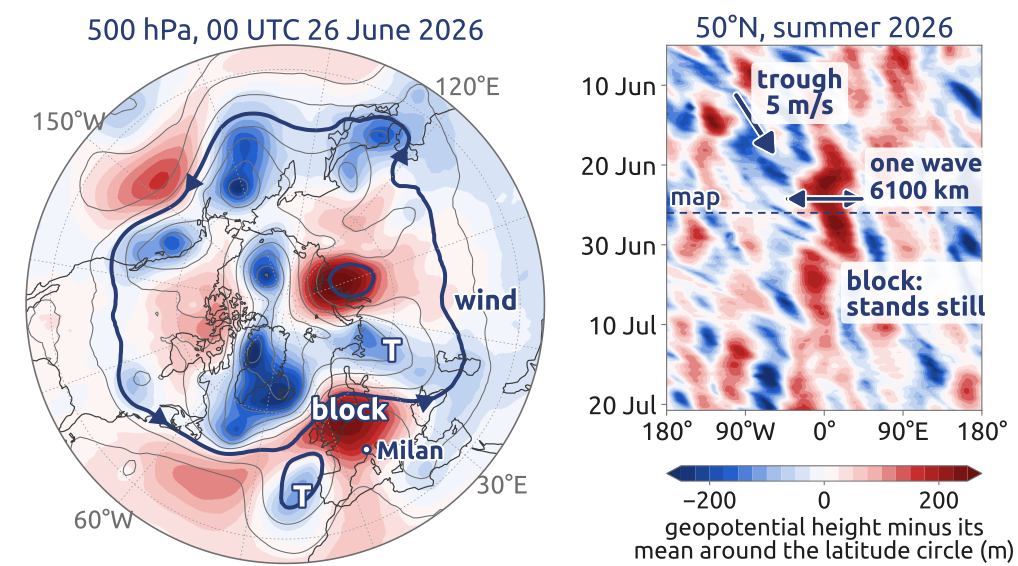
Left: 500 hPa, 00 UTC 26 June 2026; colours: geopotential height minus its latitude-circle mean (m); lines: geopotential height every 80 m (navy: 5760 m). Right: same colours at 50°N, every 6 h, longitude against time; arrows: a trough; one wave, trough to trough

ERA5 (Hersbach et al. 2020); contains modified Copernicus Climate Change Service information [2026]

June–July 2026: a ridge stood still over western Europe for three weeks (17 June–9 July), an omega between two troughs: a block; under it, western Europe’s warmest June–July on record

\[c = U - \frac{\beta}{k^2} = 0 \;\Longrightarrow\; L_s = 2\pi\sqrt{\frac{U}{\beta}} \approx 4800\ \text{km}\] \(c\): wave speed over the ground; \(U \approx 8.5\) m/s: mean eastward wind (500 hPa, 50°N, 17 June–9 July); \(\beta = df/dy = 1.5\times10^{-11}\) m\(^{-1}\)s\(^{-1}\); \(k = 2\pi/L\)

The block’s wave, about 6100 km, is about the size of \(L_s\): waves this long can stand still against the wind

But: why a block lasts for weeks, linear waves do not tell; there is no complete theory of blocking

Summer 2026: a block, a long Rossby wave standing still over western Europe for weeks

(Holton 2004, sec. 7.7.1; Woollings et al. 2018; Copernicus Climate Change Service 2026) · Data: cds.climate.copernicus.eu: ERA5 hourly data on pressure levels

Ask first: late June 2026 in Milan: which colour sat over us, and for how long? 26 June: ridge at 54°N 10°E, the 5760 m line an omega. C3S: western Europe’s warmest June–July (+2.79 °C), “atmospheric blocking”, hot air from North Africa. By the formula a 6100 km wave in 8.5 m/s drifts west at 5 m/s: same scale, not exact (the formula ignores the wave’s north–south extent). Hovmöller saw a block in his first diagram: a ridge near 0° all November 1945. Next: forecasting these slow waves: Charney (1948).

Charney (1948): keep the slow waves only

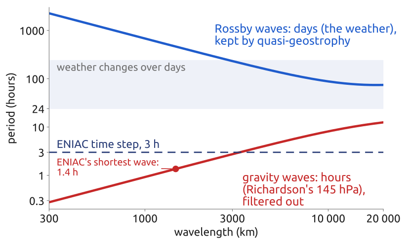
Waves in one layer of air at 45°N, no wind: period against wavelength

• The same equations carry gravity waves (hours) and Rossby waves (days); the weather is the slow kind
• Charney: with the wind nearly geostrophic and the air hydrostatic, the quasi-geostrophic equations keep only the Rossby waves

\[\underbrace{\frac{D}{Dt}\Big(\zeta + f - \frac{\psi}{L_d^2}\Big) = 0}_{\text{quasi-geostrophic, one layer}}\] \[\Big\downarrow \;\; \text{no divergence (scales} \ll L_d\text{)}\] \[\underbrace{\frac{D}{Dt}(\zeta + f) = 0}_{\text{Rossby's barotropic vorticity equation}}\]

\(\psi\): streamfunction, \(\zeta = \nabla^2\psi\); \(L_d = c/f\): deformation radius (\(c\): gravity-wave speed), about 3000 km

But: a million multiplications: a machine?

Scale analysis: drop what is small at large scales, and the fast waves go away

(Charney 1948; Lynch 2008b, sec. 2.2; Charney et al. 1950, 245)

Ask first: with a 3-hour step, can a computer follow a wave with a 1.4-hour period? Graph: linear shallow water, one layer, 45°N, c = 300 m/s, L_d = c/f ≈ 2900 km: red ω² = f² + c²k²; blue |ω| = βk/(k² + 1/L_d²) (ω < 0: westward), the quasi-geostrophic relation. L_d here: one layer, the whole depth (external); the internal L_d = NH/f of the stratified atmosphere is about 1000 km (lecture 3). ψ: streamfunction (u = −ψ_y, v = ψ_x). CFL (1928): an explicit step must not outrun the fastest wave (lecture 5). Baroclinic instability: Charney (1947), Eady (1949).

The first computer forecast (1950)

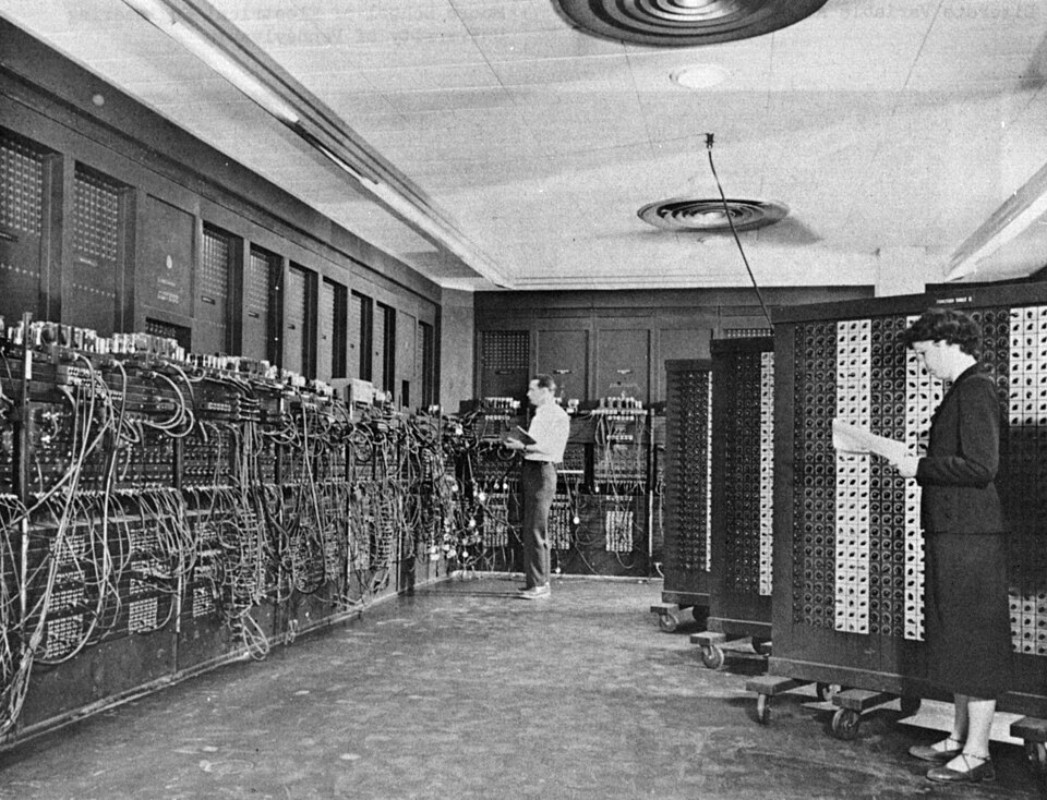
The ENIAC at Aberdeen, programmed by Glen Beck and Betty Snyder. U.S. Army photo, public domain

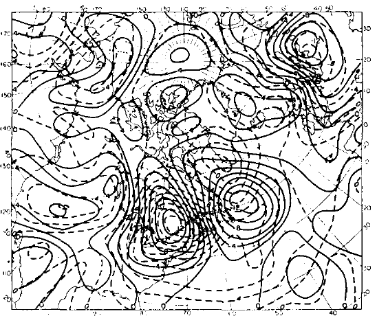
24-h change of 500 hPa geopotential height, 30 Jan. 1949: observed (solid), computed (dashed). CC BY 4.0

Charney, Fjørtoft and von Neumann: Rossby’s barotropic vorticity equation for the 500 hPa level, 736 km grid, 3-hour steps; 24 hours of computing for a 24-hour forecast

\[\frac{\partial\zeta}{\partial t} + J(\psi, \zeta + f) = 0\] \[\zeta = \nabla^2\psi: \text{ each step solves for the wind}\]

\(\zeta\): vorticity; \(J(\psi, q)\): advection of \(q\) by the wind; \(f\): Coriolis parameter; \(\psi\): streamfunction, \(u = -\partial_y\psi\), \(v = \partial_x\psi\)

Princeton, 1946: after the war, von Neumann (on the atomic bomb at Los Alamos from 1943) chose weather for his new computer: a Navy-funded Meteorology Project, wartime-trained scientists, Charney leading from 1948

1950: the first forecast by numbers that worked, with one equation for one layer of air

(Charney et al. 1950; Lynch 2008a; Thompson 1983; Lewis 2021) · Photo: commons.wikimedia.org: ENIAC · Map: doi:10.3402/tellusa.v2i4.8607, Fig. 3c

Ask first: 24 hours of computing for a 24-hour forecast: was it worth it? psi: streamfunction (u = −psi_y, v = psi_x); J(psi, q): the advection of q by that wind. Each step: zeta forward in time, then a Poisson problem for psi (lectures 3, 7). The ENIAC, built for the Army, started in December 1945 with “an urgent problem from Los Alamos” (Platzman 1979). Mixed results: the paper calls the 5 January forecast poor, this one good. Next: Sverdrup, Stommel, Munk. And the oceans?

Sverdrup, Stommel, Munk: the wind-driven gyres

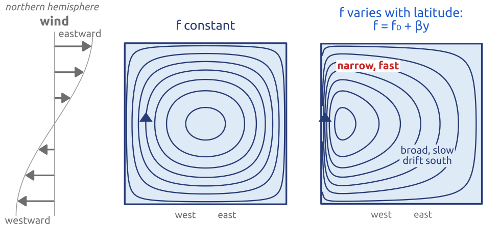
Sverdrup (1947): the wind’s spin, against \(\beta = df/dy\) (how fast \(f\) grows to the north), sets the slow drift of the interior

\[\beta V = \frac{\mathbf{k}\cdot\nabla\times\boldsymbol{\tau}}{\rho_0}\]

\(V\): northward transport; \(\boldsymbol{\tau}\): wind stress; \(\rho_0\): density of sea water; \(\mathbf{k}\cdot\nabla\times\): spin (curl)

Stommel (1948): with \(\beta\), the return flow is narrow and fast, along the ocean’s western side, off America: the Gulf Stream. Munk (1950): real winds, real transports

The same \(\beta\): the weather’s waves drift west, the Gulf Stream hugs the ocean’s western side

(Sverdrup 1947; Stommel 1948; Munk 1950; Vallis 2017, sec. 19.1)

Ask first: the westward trade winds and the eastward winds further north spin the North Atlantic clockwise: where is the return flow? The answer to the Ekman slide’s question. V: northward transport per unit width; tau: wind stress. The figure is Stommel’s model redrawn (bottom friction); without beta the gyre is symmetric. Next: Bryan and Cox, the ocean by numbers (1960s).

Bryan, Cox (1960s): the ocean by numbers

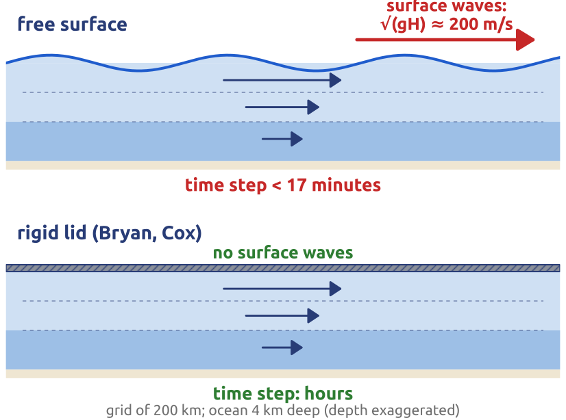
• 1960: GFDL starts a model of the world ocean (Kirk Bryan, Michael Cox): “a fool’s mission” for many
• The trick: a rigid lid removes the fast surface waves, so the step can be long, as Charney’s filter did for the air
• Manabe and Bryan (1969): ocean and atmosphere coupled: the first climate model

\[\begin{aligned} &\text{momentum:} && \frac{D\mathbf{u}_h}{Dt} + f\,\mathbf{k}\times\mathbf{u}_h = -\frac{1}{\rho_0}\nabla_h p + \mathbf{F}\\[2pt] &\text{hydrostatic balance:} && \frac{\partial p}{\partial z} = -\rho g\\[2pt] &\text{continuity (Boussinesq):} && \nabla\cdot\mathbf{u} = 0, \qquad \text{rigid lid: } w = 0 \text{ at the top}\\[2pt] &\text{heat, salt, state:} && \frac{DT}{Dt} = \dot T, \quad \frac{DS}{Dt} = \dot S, \quad \rho = \rho(T, S, p) \end{aligned}\]

\(\mathbf{u}_h\): horizontal current; \(\rho_0\): mean density of seawater; \(\mathbf{F}\): friction; \(T\): temperature; \(S\): salinity; \(\dot T\), \(\dot S\): sources by turbulent mixing, not time derivatives (surface fluxes: boundary conditions)

The ocean followed the air: first models in the 1960s, with the fast waves filtered out

(Bryan 1969, 349–51; Randall et al. 2019, sec. 4a; Manabe and Bryan 1969)

Ask first: ocean currents move at cm/s; why would an ocean model need steps of minutes? (Surface waves, 200 m/s.) “A fool’s mission”, “the first true climate model”: Randall et al. (2019). Manabe: Nobel Prize in Physics 2021. Manabe and Bryan (1969): 5 ocean levels, ~500 km grid, idealized basin; T, S and a realistic equation of state; 1 atmospheric year coupled to 100 ocean years; 1200 hours on a UNIVAC 1108. Then: B grid and Arakawa’s scheme; eddies resolved globally only in 1992 (Semtner and Chervin); today: lecture 9. Next: the whole story on one timeline.

Timeline: to weather and ocean models

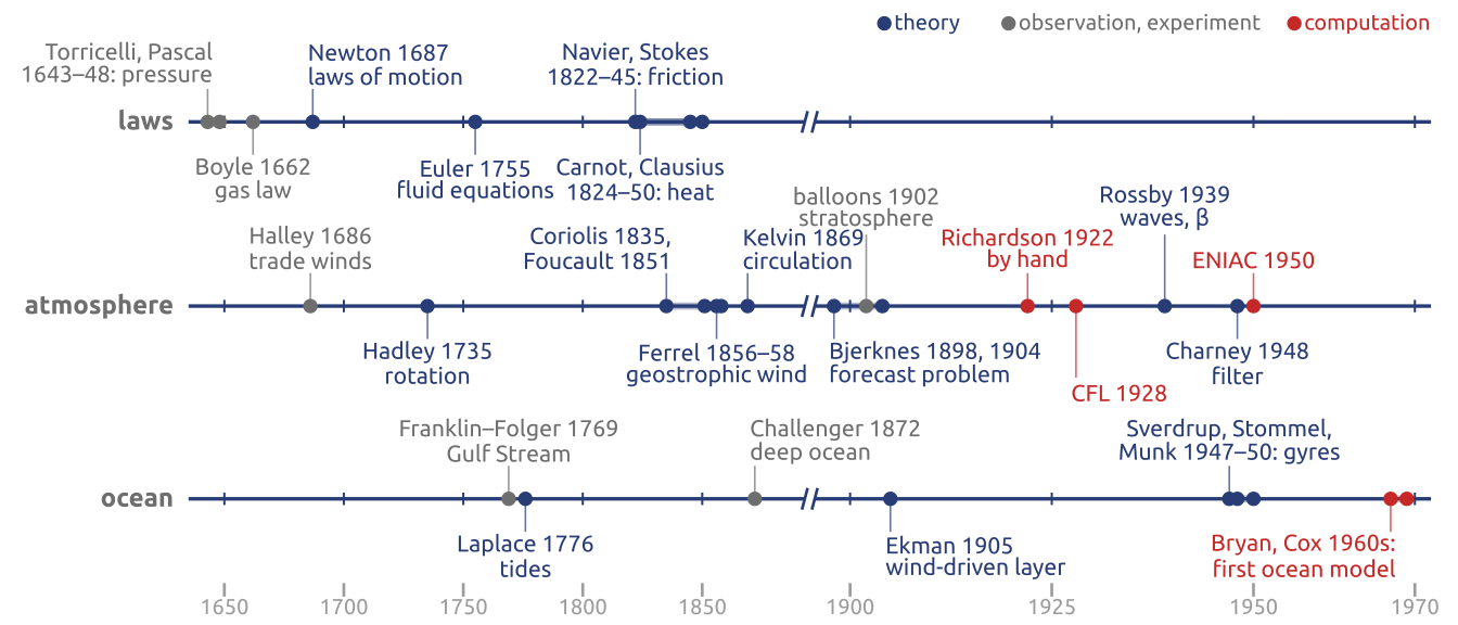
By the 1960s: the physics, and the first computed atmosphere and ocean, the roots of today’s models

(Vallis 2016; Lynch 2008b)

Ask first: which step of today’s story was the hardest, and why? Explained: rotation turns the flow (f, geostrophy); density differences start it; with beta, waves drift west and currents hug western coasts; with the fast waves filtered, a forecast by numbers works. Open: the full equations with their fast waves (balance, stable steps); the vertical, the deep ocean; the whole sphere, at fine resolution, fast enough to be useful. These open points are the course: lectures 2-3 the full equations, 4 the vertical, 5-6 stable steps and conservation, 7-9 the sphere and today’s models. Next: a weather model today.

A weather model today

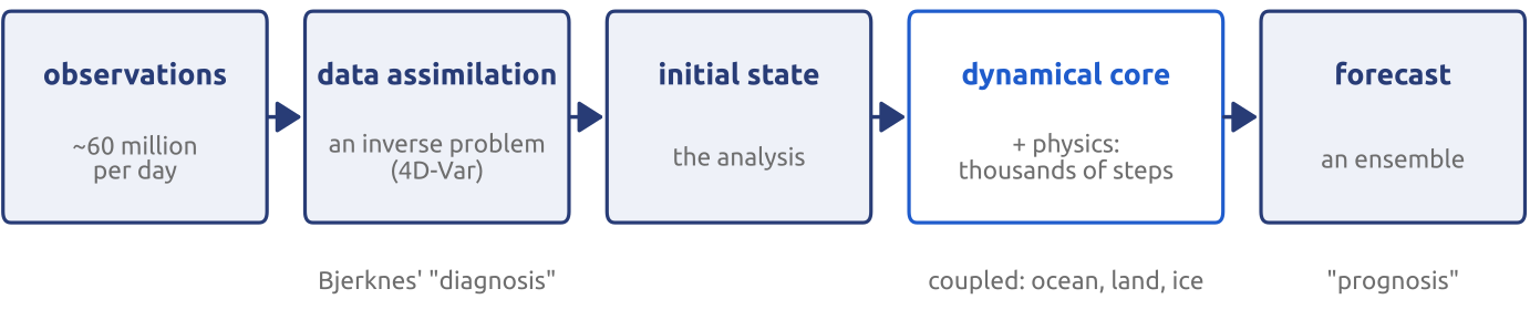
• 1950: one equation, one layer of air, a 736 km grid over North America; a day of computing for a day of forecast

• Today: the full equations on the whole globe, ~10 km, ~100 levels, coupled to ocean, land and ice; observations assimilated; ensembles; minutes of computing

Bjerknes’ plan, Richardson’s method; inside the dynamical core, the giants’ laws

(Bauer et al. 2015; Kalnay 2003; Lynch 2008b, secs. 1.2–1.3)

Lynch (2008): Richardson’s scheme “a precise and detailed implementation of the prognostic component of Bjerknes’ program”; today’s algorithms are “remarkably similar to Richardson’s scheme”. Roadmap slide: each box is a later part of the course (dynamical core: lectures 2-8; the chain: lecture 9). Next: the equations of a geophysical fluid.

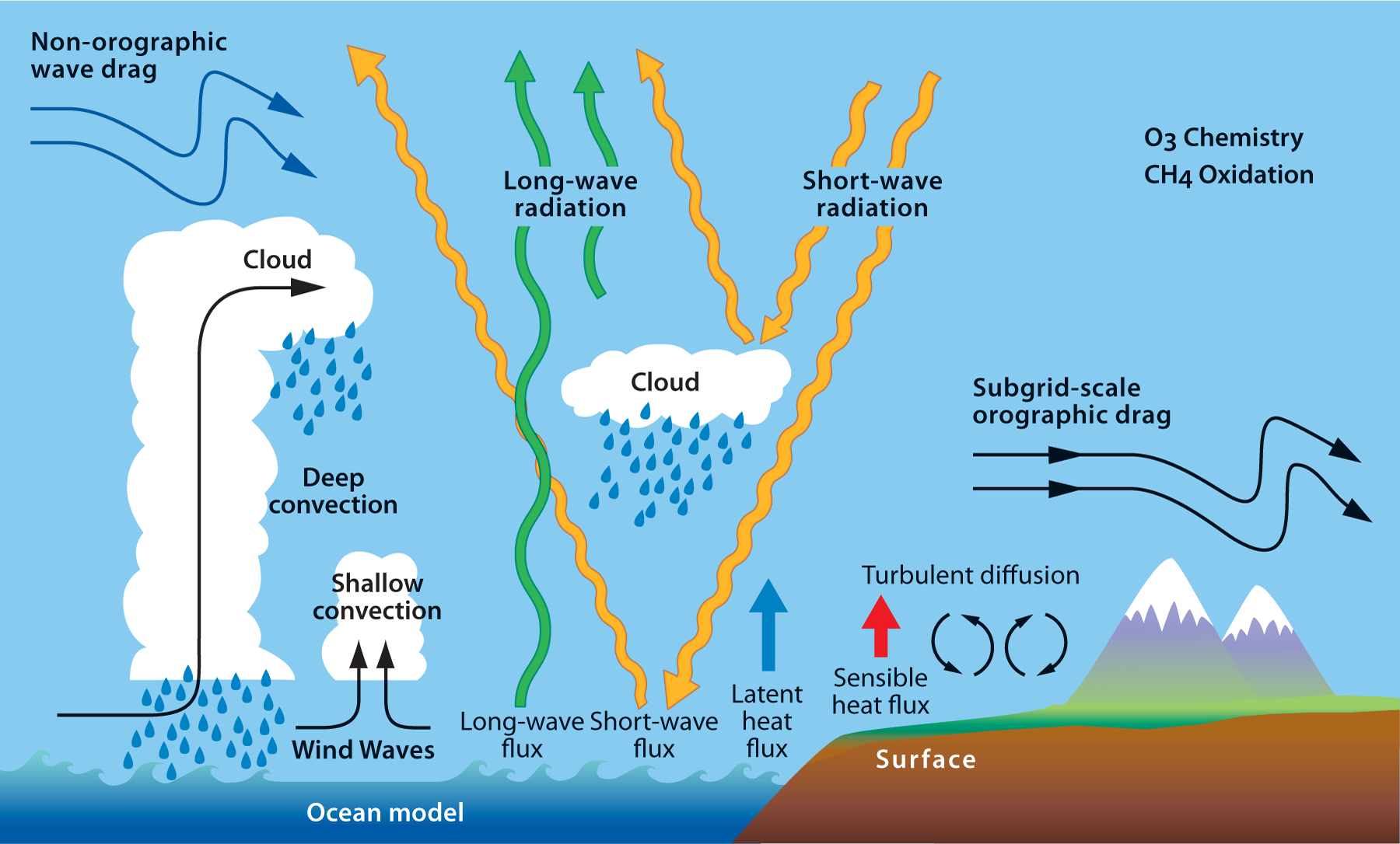
Operational weather forecast model

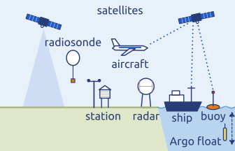
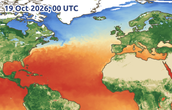
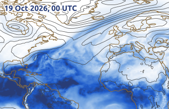
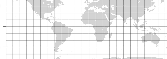
Data

Physics
Parameterization

Forcings
ocean, land, ice

Assimilation
to model space

Initial Conditions

Dynamical core
(Euler/Navier–Stokes)
Advance time

Forecast

ECMWF, CC BY 4.0

At the start: sea-surface (skin) temperature, −2 (blue) to 30 °C (red); topsoil water, dry (sand) to wet (green); sea ice and snow, white

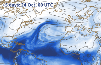
Initial conditions and forecast: total column water vapour, 5 (white) to 60 kg m⁻² (navy); lines: mean sea-level pressure every 8 hPa. All three maps: one run of the ECMWF IFS, 19 Oct 2026, 00 UTC (step 0 and +120 h), North Atlantic and Europe; drawn from ECMWF open data, CC BY 4.0

(Kalnay 2003) · Data: after wmo.int: Global Observing System · Physics: ecmwf.int: Atmospheric physics · Maps: ecmwf.int: Open data

Roadmap slide: each box is a later part of the course (data assimilation, dynamical cores, parameterizations, coupling). Inside the dynamical core: the laws the giants found (next slides). The maps are one real forecast (ECMWF, 19 Oct 2026): its start, five days later, and the surface below it.

The equations of motion

\[\underbrace{\frac{D\mathbf{u}}{Dt}}_{\text{Newton, Euler}} + \underbrace{2\boldsymbol{\Omega}\times\mathbf{u}}_{\text{Coriolis}} = \underbrace{-\frac{1}{\rho}\nabla p}_{\text{Euler, Torricelli}} \underbrace{-\,\nabla\Phi}_{\text{gravity}} + \underbrace{\nu\nabla^2\mathbf{u}}_{\text{Navier, Stokes}}\]

\[\underbrace{\frac{D\rho}{Dt} + \rho\,\nabla\cdot\mathbf{u} = 0}_{\text{continuity (Euler)}} \qquad \underbrace{p = \rho R T}_{\text{ideal gas law}}, \quad \underbrace{c_p\frac{DT}{Dt} - \frac{1}{\rho}\frac{Dp}{Dt} = Q}_{\text{first law}} \qquad \underbrace{\frac{Dq}{Dt} = \dot q}_{\text{water vapour}}\]

\(\mathbf{u} = (u, v, w)\): velocity; \(D/Dt\): rate of change following the fluid; \(\boldsymbol{\Omega}\): Earth’s rotation; \(\rho\): density; \(p\): pressure; \(\Phi\): geopotential; \(\nu\): viscosity; \(T\): temperature; \(c_p\): specific heat; \(R\): gas constant; \(Q\): heating; \(q\): water vapour; \(\dot q\): its sources (the dot names a source, not a time derivative)

• Seven unknowns \(u, v, w, p, \rho, T, q\); seven equations: Bjerknes’ programme (1904)
• The ocean: salinity instead of water vapour, and the equation of state of seawater

To be shown: the derivation of these equations from Newton’s laws, on the rotating Earth

(Bjerknes 1904; Vallis 2017)

The whole of today in two lines: each term has its giant. D/Dt: following the parcel. Omega: the Earth’s rotation. Phi: gravity plus the centrifugal force. Q: heating; q-dot: sources and sinks of vapour (evaporation, condensation).

A preview: the primitive equations

\[\frac{D\mathbf{u}_h}{Dt} + f\,\mathbf{k}\times\mathbf{u}_h = -\frac{1}{\rho}\nabla_h p + \mathbf{F}\] \[\underbrace{\frac{\partial p}{\partial z} = -\rho g}_{\text{hydrostatic balance}}\]

\(\mathbf{F}\): friction; \(p\): pressure; \(\rho\): density; \(g\): gravity; \(\nabla_h\): horizontal gradient

• Thin shell: the vertical equation becomes hydrostatic balance; rotation enters through \(f\); \(\mathbf{u}_h = (u, v)\) is the horizontal wind
• With mass, heat and the gas law: the primitive equations
• Richardson solved them by hand (1922); most climate models, and ocean models (with Boussinesq), still solve them

Thin and hydrostatic: the primitive equations, the core of weather, ocean and climate models

(Vallis 2017; Richardson 1922)

Derived in lecture 3 by scale analysis. F: friction and the other forces. Kilometre-scale models drop the hydrostatic approximation (lectures 4 and 9). The ocean: Boussinesq (density nearly constant except in the buoyancy).

Key points

1. The rotation felt locally: \(f = 2\Omega\sin\varphi\), about \(10^{-4}\ \mathrm{s^{-1}}\) at Milan; moving air turns right in the northern hemisphere
2. Geostrophic balance: the wind blows along the isobars, low pressure on its left (northern hemisphere)
3. Rossby number \(Ro = U/(fL)\): rotation matters when \(Ro \lesssim 1\)
4. Spin: circulation and vorticity; \(\zeta + f\) is kept, and \(f\) grows to the north (\(\beta\))
5. A forecast is an initial-value problem; fast waves and balance decide whether it works
6. The equations: Navier–Stokes on the rotating Earth, mass, heat; thin shells are hydrostatic (the primitive equations)

Notebook 01 (open in Colab · download): exercises 1 and 2 come back there. We suggest you run this notebook as soon as possible to test your Python environment.

Behind all of this: Newton’s laws for a fluid on the rotating Earth

(Vallis 2017; Cushman-Roisin and Beckers 2011)

Tomorrow: the equations behind all of this, from Newton’s laws; its warm-up asks about these six.