The equations of motion from basic principles
Atmosphere and Ocean Dynamics, Lecture 2: notes
The equations of motion of a fluid on the rotating Earth, derived term by term. These notes discuss fluid parcels, the Lagrangian and Eulerian descriptions and the material derivative; mass conservation, in flux form and for a parcel; Newton’s second law for a parcel, Euler’s and the Navier–Stokes equations; the Coriolis and centrifugal forces seen from the turning Earth, and the geopotential; the momentum equation in spherical coordinates; and the gas law, the first law, potential temperature and the equation of state of seawater, which close Bjerknes’ seven equations.
1 The equations of motion
The slide shows the equations that weather, ocean and climate models solve, each term labelled with the name it is known by: \[ \begin{gathered} \frac{D\mathbf{u}}{Dt} + 2\boldsymbol{\Omega}\times\mathbf{u} = -\frac{1}{\rho}\nabla p - \nabla\Phi + \nu\nabla^2\mathbf{u},\\ \frac{D\rho}{Dt} + \rho\,\nabla\cdot\mathbf{u} = 0, \qquad p = \rho R T, \qquad c_p\frac{DT}{Dt} - \frac{1}{\rho}\frac{Dp}{Dt} = Q, \qquad \frac{Dq}{Dt} = \dot q . \end{gathered} \] Here \(\mathbf{u} = (u, v, w)\) is the velocity relative to the Earth (east, north, up), \(D/Dt\) the rate of change following the fluid, \(\boldsymbol{\Omega}\) the Earth’s rotation vector, \(\rho\) the density, \(p\) the pressure, \(\Phi\) the geopotential, \(\nu\) the kinematic viscosity, \(T\) the temperature, \(R\) the gas constant, \(c_p\) the specific heat at constant pressure, \(Q\) the heating rate per unit mass, \(q\) the specific humidity (mass of water vapour per unit mass of air) and \(\dot q\) its sources and sinks (evaporation, condensation). The dot names a source term (Vallis 2017, sec. 1.2, eq. 1.41): \(\dot q\) is what changes \(q\) along a parcel, given by the physics (here condensation and evaporation); by the equation it equals \(Dq/Dt\), but it is not a time derivative computed from \(q\). The momentum equation is Newton’s law for a fluid (Newton, Euler), seen from the rotating Earth (Coriolis), pushed by pressure differences (Torricelli, Euler), gravity, and friction (Navier, Stokes); the second line holds mass conservation (Euler), the gas law and the first law of thermodynamics.
In 1904 Vilhelm Bjerknes stated weather forecasting as an initial-value problem: know the state of the atmosphere at one time, and the laws by which one state develops from another (Bjerknes 1904, transl. p. 664). The state is seven fields, \(u, v, w, p, \rho, T, q\), and he counted seven equations from laws all known in 1904: Newton’s second law (three components), the conservation of mass, the equation of state, the first law of thermodynamics and the conservation of water. In the ocean, salinity takes the place of water vapour, and an empirical equation of state of seawater that of the gas law (Cushman-Roisin and Beckers 2011, sec. 3.6). Two things make the derivation more than a restatement of Newton’s mechanics: a fluid moves and deforms, so we must say what a “body” is and what its time derivative means; and we observe it from a rotating planet (Vallis 2017, Ch. 1–2).
2 Fluid parcels
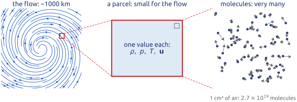
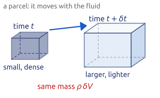
A cubic centimetre of air at sea level holds about \(2.7\times10^{19}\) molecules, which travel about \(0.07\ \mu\mathrm{m}\) between collisions. Nobody follows molecules. A fluid parcel is a volume of fluid small compared with the scales of the flow (for a cyclone 1000 km across, a parcel of 1 km is small), but large compared with the molecular scales, so that it holds very many molecules and has a well-defined density, pressure, temperature and velocity, averages over its molecules (Figure 1). The continuum hypothesis is that these averages vary smoothly from parcel to parcel, so that the state of the fluid is a set of fields, \(\rho(\mathbf{x}, t)\), \(p(\mathbf{x}, t)\), \(T(\mathbf{x}, t)\), \(\mathbf{u}(\mathbf{x}, t)\), with \(\mathbf{x} = (x, y, z)\) the position (Vallis 2017, sec. 1.1; Holton 2004, sec. 1.1). It holds very well in the ocean and in the atmosphere below about 100 km, and fails only in the very thin upper atmosphere. A parcel is made of the same molecules as it moves (molecular diffusion aside): it is a body, and Newton’s laws apply to it. Vallis calls the infinitesimal limit a fluid element, “effectively a very small fluid parcel of fixed mass” (Vallis 2017, sec. 1.1.2).
3 Two views: Lagrangian and Eulerian
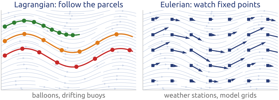
There are two ways to describe a flow (Figure 2). In the Lagrangian (material) description we follow each parcel: its position \(\mathbf{x}(t)\) and its properties along its path, \(T(t)\), \(\rho(t)\). Balloons drifting with the wind and drifting buoys measure in this way, and so do particle methods in computing. In the Eulerian (field) description we give the fields at fixed points, \(T(\mathbf{x}, t)\), \(\mathbf{u}(\mathbf{x}, t)\): weather stations, moored current meters, most satellite products and most model grids work this way (Vallis 2017, sec. 1.1.1; Cushman-Roisin and Beckers 2011, App. A.1). Both views were used by both Euler and Lagrange; the names are conventions. The physical laws are simplest for parcels, which have a mass, an acceleration and a heat budget; observations and models are mostly Eulerian. The link between them is the material derivative.
A question to test the difference: at night a weather station sees the temperature drop by 2 K in an hour. Did the air over it cool by 2 K? Not necessarily: colder air may be blowing in.
4 Material derivative (1/2): follow the parcel
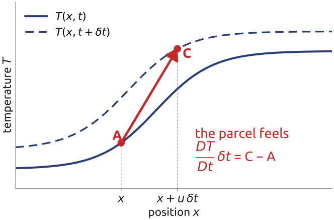
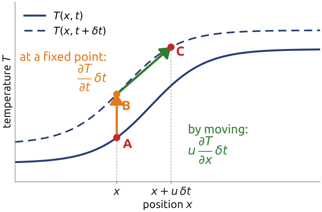
Take a parcel that is at \(\mathbf{x}\) at time \(t\). A short time \(\delta t\) later it is at \(\mathbf{x} + \mathbf{u}\,\delta t\). The change of temperature it feels is, by a Taylor expansion (the chain rule) to first order in \(\delta t\), \[ \begin{aligned} \delta T &= T(\mathbf{x} + \mathbf{u}\,\delta t,\ t + \delta t) - T(\mathbf{x}, t)\\ &\approx \frac{\partial T}{\partial t}\,\delta t + u\,\frac{\partial T}{\partial x}\,\delta t + v\,\frac{\partial T}{\partial y}\,\delta t + w\,\frac{\partial T}{\partial z}\,\delta t . \end{aligned} \] The first term is the change of the field in time at the fixed point; the other three come from moving, in \(\delta t\), through a field that varies in space. Figure 3 shows it in one dimension. Dividing by \(\delta t\) and letting \(\delta t \to 0\) gives the rate of change following the parcel (Vallis 2017, sec. 1.1.2, eqs. 1.4–1.7; Holton 2004, sec. 2.1).
5 Material derivative (2/2): change and advection
The limit is the material derivative: \[ \frac{DT}{Dt} = \frac{\partial T}{\partial t} + \mathbf{u}\cdot\nabla T . \tag{1}\] The first term is the local change, at a fixed point; the second, the change due to motion through a field that varies in space, is advection. Figure 4 splits the change felt by the parcel (from A to C) into these two pieces: from A to B the field changes at the fixed point \(x\); from B to C the parcel moves along the new profile. The operator \(D/Dt = \partial_t + \mathbf{u}\cdot\nabla\) applies to any field, and to each Cartesian component of a vector (Vallis 2017, eqs. 1.8–1.10). The acceleration of a parcel is \[ \frac{D\mathbf{u}}{Dt} = \frac{\partial\mathbf{u}}{\partial t} + (\mathbf{u}\cdot\nabla)\mathbf{u} , \] quadratic in \(\mathbf{u}\): the nonlinearity of fluid dynamics comes from here, from the velocity carrying itself.
If the parcels keep their temperature, \(DT/Dt = 0\), a station at a fixed point records \(\partial T/\partial t = -\mathbf{u}\cdot\nabla T\): the temperature changes there only because air of another temperature is brought in, as when a cold front passes. With heating, \(DT/Dt\) is the heating rate of each parcel, and the station records the sum of heating and advection.
Mathematical aside. Along the path \(\mathbf{x}(t)\) of a parcel, \(d\mathbf{x}/dt = \mathbf{u}(\mathbf{x}, t)\), and the chain rule gives \(\frac{d}{dt}F(\mathbf{x}(t), t) = \partial_t F + \mathbf{u}\cdot\nabla F\) (Chorin and Marsden 1993, sec. 1.1): the material derivative is the time derivative following a parcel, written in Eulerian variables. Along a curve \(\mathbf{x} = \mathbf{c}(t)\) that is not a parcel path, such as the track of a ship, the rate of change is \(\partial_t F + \dot{\mathbf{c}}\cdot\nabla F\): a third kind of time derivative.
6 In class: a thermometer in the wind
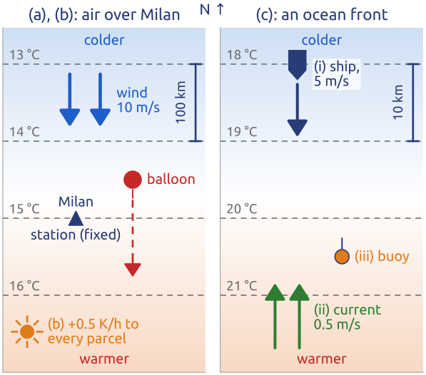
Exercise 1 — Eulerian and Lagrangian. A wind of 10 m/s blows southward over Milan; the air is colder towards the north: the temperature falls by 1 K every 100 km. (a) If each parcel keeps its temperature, how fast does the thermometer of a weather station in Milan change (K/h)? (b) The Sun now warms every parcel by 0.5 K/h. What does the station record? And a balloon drifting with the air?
Southward wind: \(v = -10\) m/s. Colder to the north: \(\partial T/\partial y < 0\) (Figure 5).
(c) A ship crossing a front. A research ship sails south at 5 m/s across an ocean front where the surface water warms by 1 K every 10 km towards the south. (i) The front does not move and there is no current: what does the ship’s thermometer record (K/h)? (ii) The ship stops; a current of 0.5 m/s flows north and carries the water with its temperature: what does it record now? (iii) And a buoy drifting with the current? Which time derivative is each one?
7 Mass (1/4): a box fixed in space
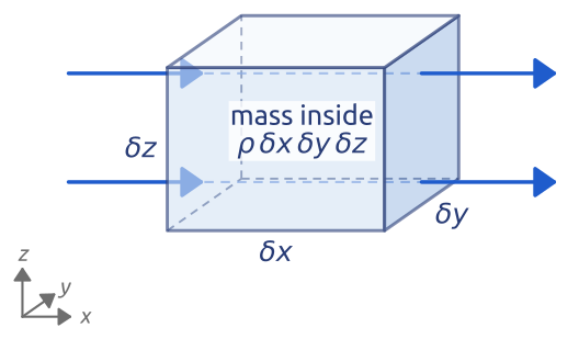
We first count the mass in a small box fixed in space, a control volume, with edges \(\delta x\), \(\delta y\), \(\delta z\) along the axes (Figure 6). The mass inside is \[ M = \rho\,\delta x\,\delta y\,\delta z , \] and mass is neither created nor destroyed: \(M\) changes only by fluid flowing in or out through the six faces, \(\partial M/\partial t = \text{inflow} - \text{outflow}\) (Vallis 2017, sec. 1.2.1; Cushman-Roisin and Beckers 2011, sec. 3.1 and App. A.1). The same bookkeeping, done for the cells of a grid, is the finite-volume method.
8 Mass (2/4): fluxes through two faces
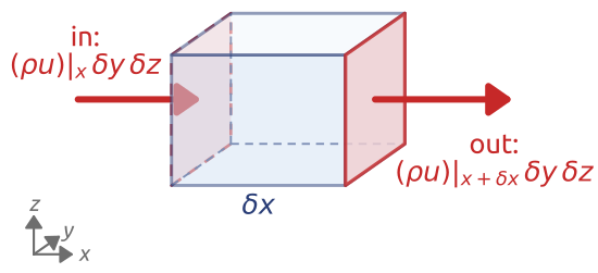
Through a face normal to \(x\), the mass that crosses per second is the density times the velocity normal to the face times the area. Per unit area, \(\rho u\) is the mass flux (kg m\(^{-2}\) s\(^{-1}\)); \((\rho u)\big|_x\) is its value on the face at \(x\) (a bar, “evaluated at”; a subscript \(x\) would mean a derivative). Through the face at \(x\) (area \(\delta y\,\delta z\)) the inflow is \((\rho u)\big|_x\,\delta y\,\delta z\); through the face at \(x + \delta x\) the outflow is \((\rho u)\big|_{x+\delta x}\,\delta y\,\delta z\) (Figure 7). A Taylor expansion across the box, to first order in \(\delta x\), \[ (\rho u)\big|_{x+\delta x} \approx (\rho u)\big|_x + \frac{\partial(\rho u)}{\partial x}\,\delta x , \] gives the net inflow through the two faces, \[ \big[(\rho u)\big|_x - (\rho u)\big|_{x+\delta x}\big]\,\delta y\,\delta z \approx -\frac{\partial(\rho u)}{\partial x}\,\delta x\,\delta y\,\delta z \] (Vallis 2017, eq. 1.23, who writes \((\rho u)(x, y, z)\)). A uniform flux brings in as much as it takes out: only the change of the flux across the box counts.
9 Mass (3/4): all six faces
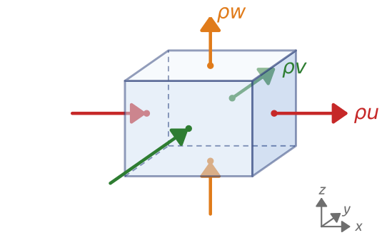
The faces normal to \(y\) and \(z\) give \(-\partial_y(\rho v)\,\delta x\,\delta y\,\delta z\) and \(-\partial_z(\rho w)\,\delta x\,\delta y\,\delta z\) (Figure 8). The volume is fixed, so \(\partial M/\partial t = (\partial\rho/\partial t)\,\delta x\,\delta y\,\delta z\); dividing by the volume, \[ \frac{\partial\rho}{\partial t} + \frac{\partial(\rho u)}{\partial x} + \frac{\partial(\rho v)}{\partial y} + \frac{\partial(\rho w)}{\partial z} = 0, \qquad\text{that is}\qquad \frac{\partial\rho}{\partial t} + \nabla\cdot(\rho\mathbf{u}) = 0 , \tag{2}\] the mass continuity equation in flux form (or conservative form) (Vallis 2017, eqs. 1.23–1.27). The three flux terms form the divergence of the mass flux, its net outflow per unit volume.
For a volume \(V\) of any size and shape, fixed in space, with boundary \(\partial V\) and outward unit normal \(\mathbf{n}\), the same bookkeeping reads \[ \frac{d}{dt}\int_V \rho\, dV = -\oint_{\partial V} \rho\,\mathbf{u}\cdot\mathbf{n}\, dA . \tag{3}\] The divergence theorem, \(\int_V \nabla\cdot\mathbf{F}\,dV = \oint_{\partial V}\mathbf{F}\cdot\mathbf{n}\,dA\) for any vector field \(\mathbf{F}\), with \(\mathbf{F} = \rho\mathbf{u}\), turns it into \(\int_V [\partial_t\rho + \nabla\cdot(\rho\mathbf{u})]\,dV = 0\); since \(V\) is arbitrary and the integrand continuous, Equation 2 follows (Vallis 2017, eqs. 1.28–1.30). The integral form is the more general: it holds even where the fields jump (fronts, shocks), where the differential form needs smooth fields. It is what the finite-volume method discretizes: cell averages updated by fluxes through the cell faces, so that what leaves one cell enters its neighbour and the total mass is conserved exactly.
10 Mass (4/4): following the parcel
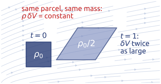
Expanding the divergence by the product rule, \(\nabla\cdot(\rho\mathbf{u}) = \mathbf{u}\cdot\nabla\rho + \rho\,\nabla\cdot\mathbf{u}\), and using Equation 1, \[ \frac{D\rho}{Dt} + \rho\,\nabla\cdot\mathbf{u} = 0 , \tag{4}\] the advective form (Vallis 2017, eq. 1.33). Following a parcel, its density changes only if the parcel expands or is compressed: \(\nabla\cdot\mathbf{u}\) is the rate at which the volume \(\delta V\) of a parcel grows, per unit volume (Section 11). A parcel that expands (\(\nabla\cdot\mathbf{u} > 0\)) becomes lighter, one that is compressed becomes denser (Figure 9). Water hardly compresses: in the ocean \(D\rho/Dt\) is small and \(\nabla\cdot\mathbf{u} \approx 0\), an incompressible flow.
11 A parcel (1/2): its volume
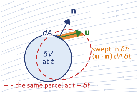
A volume \(V\) that moves with the fluid (made of the same parcels at all times) changes because its surface moves. The surface is material: each element moves with the local velocity, and in a time \(\delta t\) an element \(dA\) with outward unit normal \(\mathbf{n}\) sweeps the volume \((\mathbf{u}\cdot\mathbf{n})\,dA\,\delta t\); only the normal part of the velocity counts (Figure 10). Summing over the surface and using the divergence theorem (Vallis 2017, sec. 1.1.3, eqs. 1.12–1.13), \[ \frac{D}{Dt}\int_V dV = \oint_{\partial V}\mathbf{u}\cdot\mathbf{n}\,dA = \int_V \nabla\cdot\mathbf{u}\,dV , \] and for a small parcel of volume \(\delta V\), in the limit \(\delta V \to 0\) (Vallis’s eqs. 1.14–1.15), \[ \frac{D\,\delta V}{Dt} = \nabla\cdot\mathbf{u}\;\delta V . \tag{5}\] The same result from the edges of a small box moving with the flow: its edge \(\delta x\) is stretched at the rate \(\partial u/\partial x\) (the two ends move with velocities that differ by \(\partial_x u\,\delta x\)), and similarly for the others, so that \(\frac{1}{\delta V}\frac{D\,\delta V}{Dt} = \frac{1}{\delta x}\frac{D\,\delta x}{Dt} + \frac{1}{\delta y}\frac{D\,\delta y}{Dt} + \frac{1}{\delta z}\frac{D\,\delta z}{Dt} = \partial_x u + \partial_y v + \partial_z w\). In an incompressible flow, \(\nabla\cdot\mathbf{u} = 0\), every parcel keeps its volume.
12 A parcel (2/2): its mass
A parcel keeps its mass, \(\rho\,\delta V\). With Equation 5, \[ 0 = \frac{D(\rho\,\delta V)}{Dt} = \delta V\,\frac{D\rho}{Dt} + \rho\,\frac{D\,\delta V}{Dt} = \delta V\left(\frac{D\rho}{Dt} + \rho\,\nabla\cdot\mathbf{u}\right), \] which is Equation 4 again, now derived from the parcel’s point of view (Figure 11).
The transport theorem. Let \(\chi\) be any property per unit mass (temperature, a velocity component, a concentration). The amount of it in a parcel is \(\chi\,\rho\,\delta V\), and as \(\rho\,\delta V\) does not change, \(D(\chi\,\rho\,\delta V)/Dt = \rho\,\delta V\,D\chi/Dt\). Summed over the parcels of a volume \(V\) that moves with the fluid (Vallis 2017, sec. 1.1.3, eqs. 1.20–1.21; the name transport theorem is that of Chorin and Marsden 1993, sec. 1.1, p. 10), \[ \frac{D}{Dt}\int_V\rho\,\chi\,dV = \int_V\rho\,\frac{D\chi}{Dt}\,dV : \tag{6}\] the amount of \(\chi\) in a moving piece of fluid changes only as \(\chi\) changes along each parcel. With \(\chi = 1\) the mass of \(V\) is constant; with \(\chi = \mathbf{u}\) it gives the momentum of a finite piece of fluid.
Mathematical aside: the flow map. Chorin and Marsden (1993, sec. 1.1, pp. 7–11) derive the same results with the flow map: their \(\varphi(\mathbf{x}, t)\) is the position at time \(t\) of the parcel that was at \(\mathbf{x}\) at \(t = 0\) (a map, not the latitude used below), and \(J(\mathbf{x}, t)\) is its Jacobian determinant, the ratio of a parcel’s volume to its initial volume. They show that \(\partial J/\partial t = J\,\nabla\cdot\mathbf{u}\); that \(\rho(\varphi(\mathbf{x}, t), t)\,J(\mathbf{x}, t) = \rho(\mathbf{x}, 0)\), the Lagrangian form of mass conservation; and the transport theorem, by changing variables to the initial positions. If \(\mathbf{u}\) is Lipschitz in \(\mathbf{x}\), every parcel has a unique path and parcels never split or merge; if \(\nabla\cdot\mathbf{u} = 0\), \(J \equiv 1\) and the flow map keeps volumes.
13 The continuity equation: two views
The slide sets the two derivations side by side. Fixed in space (Eulerian; the box of Figure 8), mass changes by what flows through the faces: the flux form Equation 2 and its integral form Equation 3, with \(\partial/\partial t\) at a fixed point and \(V\) fixed. Following a parcel (Lagrangian; Figure 11), mass is kept and the volume grows at the rate \(\nabla\cdot\mathbf{u}\): the advective form Equation 4 and its integral form \[ \frac{D}{Dt}\int_V\rho\,dV = 0 , \] with \(D/Dt\) following the parcel and \(V\) moving with the fluid (Vallis 2017, sec. 1.2, eqs. 1.27 and 1.33–1.34). They are one law, linked by \(D/Dt = \partial_t + \mathbf{u}\cdot\nabla\) and \(\nabla\cdot(\rho\mathbf{u}) = \mathbf{u}\cdot\nabla\rho + \rho\,\nabla\cdot\mathbf{u}\). The flux form is what finite volumes discretize (exact conservation in each cell); the advective form is what a parcel feels, and what Lagrangian and semi-Lagrangian schemes use.
14 Momentum (1/4): Newton for a parcel
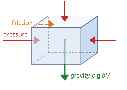
For a parcel of mass \(\rho\,\delta V\), Newton’s second law reads \[ \rho\,\delta V\,\frac{D\mathbf{u}}{Dt} = \text{body forces} + \text{surface forces} \] (the transport theorem Equation 6 with \(\chi = \mathbf{u}\) makes it precise for a finite volume). The acceleration is the material derivative, the parcel’s, not the change at a fixed point (Vallis 2017, sec. 1.3; Cushman-Roisin and Beckers 2011, sec. 3.2). Body forces act on all the mass of the parcel and are proportional to its volume: gravity, \(\rho\,\mathbf{g}\,\delta V\), with \(\mathbf{g}\) the gravity per unit mass. Surface forces act on its faces and are proportional to their area: the pressure, normal to each face, and friction (viscous stresses), along the faces (Figure 12).
15 Momentum (2/4): the pressure force
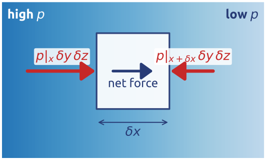
Pressure pushes each face of the box inwards, with a force equal to the pressure times the area (Figure 13). On the face at \(x\) it pushes in the \(+x\) direction with \(p\big|_x\,\delta y\,\delta z\); on the face at \(x + \delta x\) in the \(-x\) direction with \(p\big|_{x+\delta x}\,\delta y\,\delta z\). With the same Taylor step as for the mass flux, the net force in \(x\) is \[ \big[p\big|_x - p\big|_{x+\delta x}\big]\,\delta y\,\delta z \approx -\frac{\partial p}{\partial x}\,\delta x\,\delta y\,\delta z , \] and similarly in \(y\) and \(z\): the pressure force on the box is \(-\nabla p\,\delta V\), and per unit mass (dividing by \(\rho\,\delta V\)) \[ -\frac{1}{\rho}\nabla p . \] In integral form, the pressure force on a volume \(V\) is \(-\oint_{\partial V}p\,\mathbf{n}\,dA = -\int_V\nabla p\,dV\), by the divergence theorem applied to each component (Vallis 2017, sec. 1.3.2, eqs. 1.45–1.47; Holton 2004, sec. 1.4). A uniform pressure, however large, gives no net force: the atmosphere presses on us with about 10 tonnes per square metre, equally from all sides. Only pressure differences push, from high to low pressure; Vallis calls it the pressure-gradient force.
16 Momentum (3/4): gravity and friction
Gravity is a body force, \(\mathbf{g} = -g\,\mathbf{k}\) per unit mass, with \(\mathbf{k}\) the upward unit vector and \(g \approx 9.81\) m/s\(^2\). It is the gradient of a potential, \(\mathbf{g} = -\nabla\Phi\), with the geopotential \(\Phi = gz\) (\(z\): height), the potential energy per unit mass. The \(g\) we measure is the Earth’s gravitational attraction plus a small part, at most 0.35 %, from the Earth’s turning: the centrifugal force, made exact in Section 22.
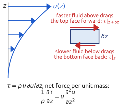
Friction acts through viscous stresses on the faces of the parcel. Take a flow \(u(z)\) along \(x\) that grows with height (Figure 14). The faster fluid above drags the top face of a box forward, the slower fluid below drags its bottom face back. For a Newtonian fluid such as air or water the stress (force per unit area) is proportional to the shear, \(\tau = \rho\nu\,\partial u/\partial z\). With the same Taylor step as for the pressure, the net force on the box is \[ \big[\tau\big|_{z+\delta z} - \tau\big|_z\big]\,\delta x\,\delta y \approx \frac{\partial\tau}{\partial z}\,\delta x\,\delta y\,\delta z , \] and per unit mass, with \(\rho\) and \(\nu\) constant, \(\nu\,\partial^2 u/\partial z^2\). The two stresses differ, and the box is pushed, only if the shear changes with height. Adding the shears in the other directions, for an incompressible flow with constant viscosity, gives the viscous friction \[ \mathbf{F} = \nu\,\nabla^2\mathbf{u} \qquad (\nabla\cdot\mathbf{u} = 0), \] with the kinematic viscosity \(\nu = \mu/\rho\) (\(\mu\): dynamic viscosity): about \(1.5\times10^{-5}\) m\(^2\)/s for air and \(1.0\times10^{-6}\) m\(^2\)/s for water (Cushman-Roisin and Beckers 2011, sec. 8.1; Vallis 2017, Table 1.1, gives \(1.1\times10^{-6}\) for water). Navier (memoir read in 1822, printed 1827) and Stokes (1845) wrote this term (Navier 1827; Stokes 1845). For a compressible fluid there is an extra term in \(\nabla(\nabla\cdot\mathbf{u})\); \(\nu\nabla^2\mathbf{u}\) “is not exact, but it is in fact a good approximation for most liquids and gases” (Vallis 2017, sec. 1.3.2).
Mathematical aside. The surface force per unit area on a face with unit normal \(\mathbf{n}\) is \(\boldsymbol{\sigma}\mathbf{n}\), with the stress tensor \(\sigma_{ij} = -p\,\delta_{ij} + \tau_{ij}\); the net surface force on a volume is \(\oint\boldsymbol{\sigma}\mathbf{n}\,dA = \int\nabla\cdot\boldsymbol{\sigma}\,dV\). The balance of angular momentum of a small parcel makes \(\boldsymbol{\sigma}\) symmetric (Cushman-Roisin and Beckers 2011, App. A.1). For an incompressible Newtonian fluid \(\tau_{ij} = \mu\,(\partial u_i/\partial x_j + \partial u_j/\partial x_i)\) (Cushman-Roisin and Beckers 2011, sec. 3.7, eq. 3.18), whose divergence, with constant \(\mu\), is \(\mu\nabla^2 u_i + \mu\,\partial_i(\nabla\cdot\mathbf{u}) = \mu\nabla^2 u_i\).
How important is friction? The ratio of the advection term, \((\mathbf{u}\cdot\nabla)\mathbf{u} \sim U^2/L\), to the viscous term, \(\nu\nabla^2\mathbf{u} \sim \nu U/L^2\), is the Reynolds number (Reynolds 1883; Vallis 2017, sec. 1.11.1), \[ Re = \frac{UL}{\nu} , \] with \(U\) and \(L\) a typical speed and length. For a vortex at a bathtub drain (\(U = 0.1\) m/s, \(L = 0.5\) m), \(Re \approx 5\times10^4\); for an ocean eddy (\(0.1\) m/s, 100 km), \(Re \approx 10^{10}\); for a cyclone (10 m/s, 1000 km), \(Re \approx 7\times10^{11}\). Winds and currents have \(Re\) from about \(10^8\) to \(10^{12}\): molecular friction is negligible at large scales. The flow is turbulent, though, and small eddies carry momentum far more efficiently than molecules, above all near the ground and the sea surface. Models do not resolve these eddies; they represent their effect by parameterizations (an eddy viscosity, a boundary-layer scheme), part of the “physics” of a model. We keep a general friction term \(\mathbf{F}\).
17 Momentum (4/4): Euler and Navier–Stokes
Putting the forces together, per unit mass, \[ \frac{D\mathbf{u}}{Dt} = -\frac{1}{\rho}\nabla p - \nabla\Phi + \mathbf{F}, \qquad \frac{\partial\rho}{\partial t} + \nabla\cdot(\rho\mathbf{u}) = 0 . \tag{7}\] With \(\mathbf{F} = 0\) these are Euler’s equations of an ideal (frictionless) fluid: Newton’s law for every parcel, the pressure on a box and gravity, as Euler wrote them in a memoir read to the Berlin Academy in 1755 and printed in 1757 (Euler 1757; Chorin and Marsden 1993, sec. 1.1); Euler also wrote the continuity equation in its modern form. With \(\mathbf{F} = \nu\nabla^2\mathbf{u}\) they are the Navier–Stokes equations (Vallis 2017, sec. 1.3.2, eq. 1.48). They are four equations (three components of momentum, and mass) for five unknowns (\(u, v, w, p, \rho\)): one more relation is needed, the equation of state, which brings in the temperature, and with it thermodynamics. And they hold in a frame of reference that does not rotate, while winds and currents are measured on the turning Earth: Coriolis (1835) showed how to change frames (Coriolis 1835).
Mathematical aside. For smooth initial data the incompressible Euler and Navier–Stokes equations in three dimensions have unique smooth solutions for some time; whether smooth solutions exist for all time is open (for Navier–Stokes, one of the Clay Millennium Prize problems). In two dimensions global smooth solutions exist, thanks to the conservation of vorticity along parcels. The hydrostatic primitive equations of large-scale atmosphere and ocean models have their own theory: with viscosity, their solutions are smooth for all time (Cao and Titi 2007). See Chorin and Marsden (1993) for the mathematical theory of the Euler and Navier–Stokes equations.
18 Rotating frame (1/4): a vector on the table
Newton’s laws hold in an inertial frame, one that neither rotates nor accelerates (“seen from space”). We measure winds and currents relative to the ground, which turns with the Earth at the rate \(\Omega = 2\pi/(\text{sidereal day}) = 7.29\times10^{-5}\ \mathrm{s^{-1}}\) about the axis through the poles. The rotation is a vector \(\boldsymbol{\Omega}\) along the axis, pointing north (right-hand rule). We write \((\;)_I\) for a rate of change seen in the inertial frame (from space) and \((\;)_R\) for one seen in the rotating frame (on the table, on the Earth), as Vallis (2017, sec. 2.1.1) does.
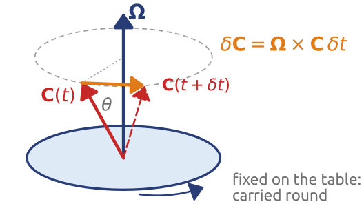
A vector \(\mathbf{C}\) fixed on a table turning at \(\boldsymbol{\Omega}\), at an angle \(\theta\) from the axis, is carried round (Figure 15): its tip moves on a circle of radius \(|\mathbf{C}|\sin\theta\) at the angular rate \(\Omega\), in the direction perpendicular to both \(\boldsymbol{\Omega}\) and \(\mathbf{C}\). In a time \(\delta t\) the tip moves by \(\Omega\,|\mathbf{C}|\sin\theta\,\delta t\), the radius of the circle times the angle turned; this is the size and direction of \(\boldsymbol{\Omega}\times\mathbf{C}\,\delta t\), so (Vallis’s eq. 2.3) \[ \left(\frac{d\mathbf{C}}{dt}\right)_I = \boldsymbol{\Omega}\times\mathbf{C} . \] In particular, the unit vectors \(\mathbf{i}'\), \(\mathbf{j}'\), \(\mathbf{k}'\) drawn on the table obey \((d\mathbf{i}'/dt)_I = \boldsymbol{\Omega}\times\mathbf{i}'\), and so on.
19 Rotating frame (2/4): any vector, the velocity
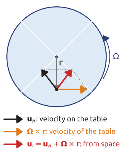
A vector that also changes on the table is written with the table’s unit vectors, \(\mathbf{B} = B_1\mathbf{i}' + B_2\mathbf{j}' + B_3\mathbf{k}'\), and differentiated in the inertial frame with the product rule. The derivatives of the components give the rate of change seen on the table, \((d\mathbf{B}/dt)_R\); the derivatives of the turning unit vectors give \(B_1\,\boldsymbol{\Omega}\times\mathbf{i}' + B_2\,\boldsymbol{\Omega}\times\mathbf{j}' + B_3\,\boldsymbol{\Omega}\times\mathbf{k}' = \boldsymbol{\Omega}\times\mathbf{B}\). So (Vallis 2017, sec. 2.1.1, eq. 2.5) \[ \left(\frac{d\mathbf{B}}{dt}\right)_I = \left(\frac{d\mathbf{B}}{dt}\right)_R + \boldsymbol{\Omega}\times\mathbf{B} . \tag{8}\] Applied to the position \(\mathbf{r}\) of a parcel, measured from a point on the axis (the centre of the Earth), \[ \mathbf{u}_I = \mathbf{u}_R + \boldsymbol{\Omega}\times\mathbf{r}, \] with \(\mathbf{u}_R = (d\mathbf{r}/dt)_R\) the relative velocity (the wind, the current) and \(\mathbf{u}_I\) the inertial velocity (Vallis 2017, sec. 2.1.2, eq. 2.7). Seen from space, a parcel moves with its velocity on the table plus the table’s own velocity there, \(\boldsymbol{\Omega}\times\mathbf{r}\) (Figure 16). On the Earth this is the ground’s speed, \(\Omega a\cos\varphi\) at latitude \(\varphi\) (\(a\): the Earth’s radius): 465 m/s at the equator, the speed in Hadley’s (1735) argument for the trade winds (Hadley 1735).
20 Rotating frame (3/4): the acceleration
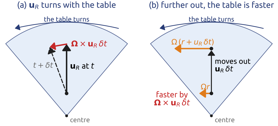
We want the acceleration seen from space, \((d\mathbf{u}_I/dt)_I\), in terms of the motion on the table, by the route of Vallis (2017, sec. 2.1.2, eqs. 2.8–2.12). Differentiate \(\mathbf{u}_I = \mathbf{u}_R + \boldsymbol{\Omega}\times\mathbf{r}\) from space, with \(\boldsymbol{\Omega}\) constant and \((d\mathbf{r}/dt)_I = \mathbf{u}_I\): \[ \left(\frac{d\mathbf{u}_I}{dt}\right)_I = \left(\frac{d\mathbf{u}_R}{dt}\right)_I + \boldsymbol{\Omega}\times\mathbf{u}_I . \] Apply Equation 8 to the relative velocity, \((d\mathbf{u}_R/dt)_I = (d\mathbf{u}_R/dt)_R + \boldsymbol{\Omega}\times\mathbf{u}_R\), and put \(\mathbf{u}_I = \mathbf{u}_R + \boldsymbol{\Omega}\times\mathbf{r}\) in the last term: \[ \begin{aligned} \left(\frac{d\mathbf{u}_I}{dt}\right)_I &= \left(\frac{d\mathbf{u}_R}{dt}\right)_R + \underbrace{\boldsymbol{\Omega}\times\mathbf{u}_R}_{\text{(a)}} + \underbrace{\boldsymbol{\Omega}\times\mathbf{u}_R}_{\text{(b)}} + \boldsymbol{\Omega}\times(\boldsymbol{\Omega}\times\mathbf{r})\\ &= \left(\frac{d\mathbf{u}_R}{dt}\right)_R + 2\,\boldsymbol{\Omega}\times\mathbf{u}_R + \boldsymbol{\Omega}\times(\boldsymbol{\Omega}\times\mathbf{r}) . \end{aligned} \tag{9}\] The Coriolis acceleration \(2\boldsymbol{\Omega}\times\mathbf{u}_R\) comes in two equal halves, drawn in Figure 17 for a parcel moving outwards from the centre of a turntable. (a) The relative velocity \(\mathbf{u}_R\) is a vector carried round by the table: even a constant \(\mathbf{u}_R\) changes direction in space, at the rate \(\boldsymbol{\Omega}\times\mathbf{u}_R\) (the rule applied to \(\mathbf{u}_R\)). (b) As the parcel moves by \(\mathbf{u}_R\,\delta t\), the velocity of the table under it, \(\boldsymbol{\Omega}\times\mathbf{r}\), changes by \(\boldsymbol{\Omega}\times\mathbf{u}_R\,\delta t\): moving outwards, it reaches a part of the table that moves faster. The last term, \(\boldsymbol{\Omega}\times(\boldsymbol{\Omega}\times\mathbf{r})\), is the centripetal acceleration of a point at rest on the table. Hadley kept the eastward speed of the air in space, which no law conserves: only the change of the ground’s speed with latitude, half (b), entered his argument, and he found half the true deflection (Persson 2006, 32; Persson 1998).
21 Rotating frame (4/4): momentum on the Earth
Newton’s law holds for the inertial acceleration, \((d\mathbf{u}_I/dt)_I\). Following a parcel, \((d\mathbf{u}_R/dt)_R\) is the material derivative computed with the relative velocity. We drop the subscript \(R\), as Vallis (2017, sec. 2.1.3) does: from now on \(\mathbf{u}\) is the velocity relative to the Earth. Moving the extra terms of Equation 9 to the right-hand side, Equation 7 becomes \[ \frac{D\mathbf{u}}{Dt} + 2\,\boldsymbol{\Omega}\times\mathbf{u} = -\frac{1}{\rho}\nabla p + \mathbf{g}_{\text{grav}} - \boldsymbol{\Omega}\times(\boldsymbol{\Omega}\times\mathbf{r}) + \mathbf{F}, \] with \(\mathbf{g}_{\text{grav}}\) Newton’s gravitational attraction of the Earth, towards its centre, in the notation of Vallis (2017, eq. 2.23). Seen from the rotating Earth, two forces per unit mass appear (Vallis 2017, eqs. 2.12–2.15). The Coriolis force \(-2\boldsymbol{\Omega}\times\mathbf{u}\) acts only on moving parcels, at right angles to their velocity: it turns them and does no work. The centrifugal force \(-\boldsymbol{\Omega}\times(\boldsymbol{\Omega}\times\mathbf{r})\) points away from the axis and acts even on a parcel at rest. Neither is a true force: Vallis calls them quasi-forces, “as if” forces felt by a body described from a rotating frame.
Mass and scalar equations (temperature, salinity, humidity) do not change: the rate of change of a scalar following a parcel is the same in both frames, and \(\nabla\cdot(\boldsymbol{\Omega}\times\mathbf{r}) = 0\), so \(\nabla\cdot\mathbf{u}_I = \nabla\cdot\mathbf{u}_R\) (Vallis 2017, sec. 2.1.4, eqs. 2.18–2.20).
We never feel the centrifugal force on its own. Why? Section 22 answers.
22 Gravity, centrifugal force, geopotential
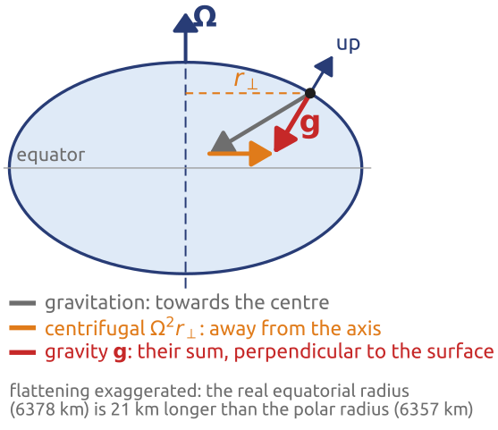
The centrifugal force is a gradient. With \(\mathbf{r}_\perp\) the vector from the axis to the parcel (at right angles to the axis, of length \(r_\perp\)), \(-\boldsymbol{\Omega}\times(\boldsymbol{\Omega}\times\mathbf{r}) = \Omega^2\mathbf{r}_\perp = -\nabla\Phi_{ce}\), with the centrifugal potential \(\Phi_{ce} = -\tfrac{1}{2}\Omega^2 r_\perp^2\) (Vallis 2017, sec. 2.1.2, eqs. 2.13–2.14). It adds to gravitation, exactly, into the effective gravity, the gradient of one geopotential \(\Phi\) (Vallis’s eqs. 2.23–2.24): \[ \mathbf{g} = \mathbf{g}_{\text{grav}} + \Omega^2\mathbf{r}_\perp = -\nabla\Phi , \] and the momentum equation in the rotating frame is (Vallis 2017, eq. 2.16, with friction) \[ \frac{D\mathbf{u}}{Dt} + 2\,\boldsymbol{\Omega}\times\mathbf{u} = -\frac{1}{\rho}\nabla p - \nabla\Phi + \mathbf{F} . \tag{10}\] The centrifugal force is kept: it is inside \(\Phi\).
Two steps are involved, and only the second is an approximation (Vallis 2017, sec. 2.2.1). First, absorbing the centrifugal force into \(\Phi\) is exact. It could not simply be dropped: it is small compared with gravity, \(\Omega^2 a/g \approx 3\times10^{-3}\) (0.034 m/s\(^2\) at the equator; Vallis’s eq. 2.25), but measured from a sphere its horizontal part is about \(\Omega a/(4U) \approx 10\) times the Coriolis force, with \(U = 10\) m/s a typical wind (his eq. 2.26). Second, “up” is taken along \(\mathbf{g}\), so that gravity has no horizontal component, and the surfaces of constant \(\Phi\) are treated, for all geometric purposes, as if they were spheres, with \(\Phi \approx gz\) and \(z\) the height above the surface of constant geopotential at sea level (the geoid). The error is geometric, of relative size \(\Omega^2 a/g\): in Vallis’s words, “we have traded a potentially large dynamical error for a very small geometric error”.
It works because the Earth has bulged until its surface is nearly a surface of constant \(\Phi\) (Figure 18). The surface of an ocean at rest must be such a surface, or water would flow along it; the solid Earth, soft over geological time, has taken nearly the same shape, an oblate spheroid whose equatorial radius (6378 km) is about 21 km longer than its polar radius (6357 km) (Cushman-Roisin and Beckers 2011, sec. 2.2; Persson 1998, 1374–75). The gravity we measure, \(\mathbf{g} = -\nabla\Phi\), is perpendicular to this surface and defines “up” and “horizontal”; it is 9.78 m/s\(^2\) at the equator and 9.83 m/s\(^2\) at the poles. Were the solid Earth an exact sphere, the ocean would pile up at low latitudes and the basins at high latitudes would dry out (Vallis 2017, sec. 2.2.1).
23 Parcels in a rotating frame
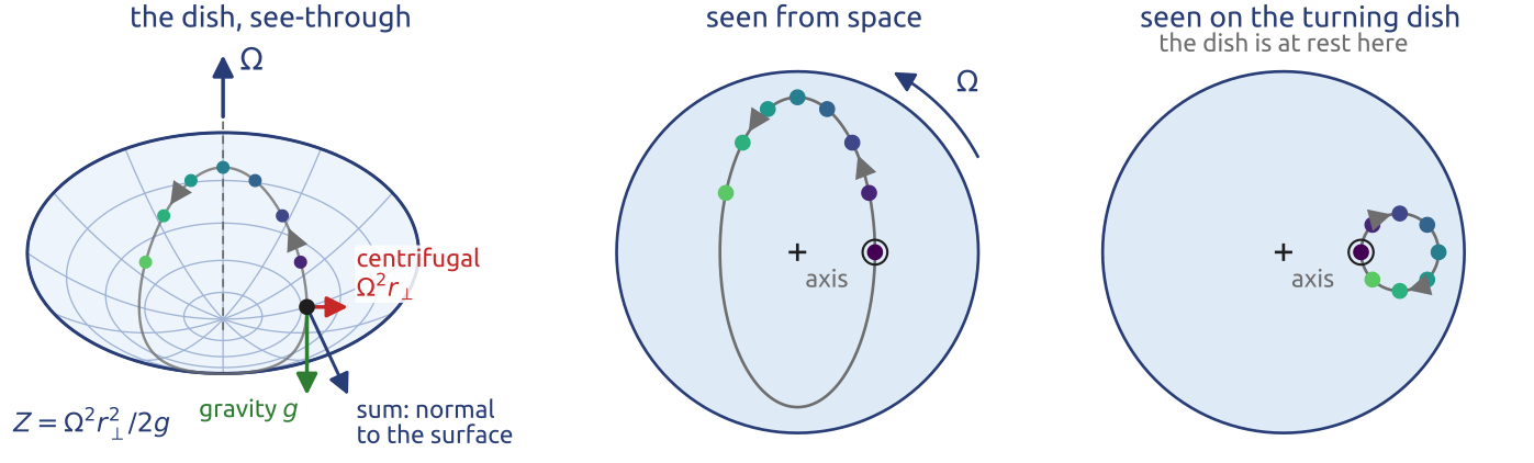
A liquid turning with its container at the rate \(\Omega\) takes the shape of a paraboloid, \[ Z = \frac{\Omega^2 r_\perp^2}{2g} , \] with \(Z\) the height of the surface and \(r_\perp\) the distance from the axis: there the slope pulls inwards, \(-g\nabla Z = -\Omega^2\mathbf{r}_\perp\), as hard as the centrifugal force \(\Omega^2\mathbf{r}_\perp\) pushes outwards, so gravity and the centrifugal force add up to a force normal to the surface. The surface is a surface of constant geopotential, \(gZ - \tfrac{1}{2}\Omega^2 r_\perp^2\), like the sea on the Earth (a tank 40 cm across at 30 turns per minute is 2 cm deeper at the rim than at the centre) (Cushman-Roisin and Beckers 2011, sec. 2.2 and §2.4, eq. 2.15). Made solid, it is a parabolic dish (Figure 19, left).
Follow a frictionless puck on a shallow dish that turns at the rate \(\Omega\). Seen from space, the only horizontal force is the slope’s pull, \[ \left(\frac{d\mathbf{u}_I}{dt}\right)_I = -\Omega^2\mathbf{r}_\perp : \] a two-dimensional harmonic oscillator of frequency \(\Omega\) (Cushman-Roisin and Beckers 2011, eqs. 2.16–2.17). Its paths are ellipses centred on the axis, run once every \(2\pi/\Omega\) (a straight swing through the axis if the puck is let go at rest). Seen on the dish, the slope’s pull and the centrifugal force cancel exactly, and only the Coriolis force is left, \[ \left(\frac{d\mathbf{u}_R}{dt}\right)_R = -2\boldsymbol{\Omega}\times\mathbf{u}_R , \qquad\text{in components}\qquad \frac{du}{dt} - f v = 0, \quad \frac{dv}{dt} + f u = 0 , \] with \(f = 2\Omega\) (Cushman-Roisin and Beckers 2011, sec. 2.3, eq. 2.11). For a puck launched northward at the speed \(V\) on the dish, the solution is \(u = V\sin ft\), \(v = V\cos ft\): the speed stays \(V\) while the direction turns, and the puck runs round an inertial circle of radius \(V/f\), clockwise on a dish turning anticlockwise, once every \(2\pi/f\), half a turn of the dish (their eqs. 2.12–2.14). Turning the ellipse with the dish gives exactly the inertial circle: one motion, two explanations. From space, the restoring force is gravity’s pull down the slope; on the dish, it is the Coriolis force (Cushman-Roisin and Beckers 2011, sec. 2.4; Durran 1993). On the Earth the oblate shape plays the part of the dish: gravity balances the centrifugal force on a body at rest, and only the Coriolis force acts on moving ones (Persson 1998, 1374–75). On the Earth \(f = 2\Omega\sin\varphi\); at Milan the inertial period \(2\pi/f\) is about 17 h.
24 Inertial circles and the geostrophic drift
Two results of the dish. From space the slope pulls the puck back to the axis, along an ellipse; on the dish, slope and centrifugal force cancel and the puck runs round an inertial circle once every \(2\pi/f\), \(f = 2\Omega\).
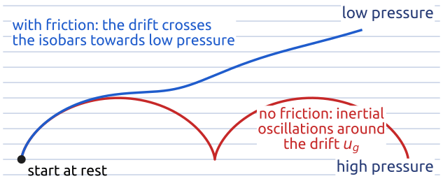
Now release a parcel at rest on the \(f\)-plane (constant \(f\)) under a uniform pressure gradient, the isobars along \(x\) (east) and the low pressure to the north: \[ \frac{du}{dt} = f v, \qquad \frac{dv}{dt} = -f u - \frac{1}{\rho}\frac{\partial p}{\partial y} . \] It is first pushed towards low pressure, then turned to the right (northern hemisphere) by the Coriolis force. With \(u_g = -(\rho f)^{-1}\,\partial p/\partial y\), the second equation reads \(dv/dt = -f(u - u_g)\): in a frame drifting eastward at \(u_g\) the parcel only feels the Coriolis force, so its path is an inertial circle carried along at \(u_g\), a cycloid. The exact solution from rest is \(u = u_g(1 - \cos ft)\), \(v = u_g\sin ft\): inertial loops of radius \(u_g/f\) around a drift along the isobars at the geostrophic speed \(u_g\), with the low pressure on its left (Figure 20). Ferrel’s geostrophic wind (Ferrel 1858) is the average motion; the oscillations around it are inertial.
With a linear drag \(-\epsilon\,\mathbf{u}\) (\(\epsilon\): a constant rate), the crudest model of turbulent friction near the ground, the loops die out and the parcel settles into a steady drift in which three forces balance: pressure, Coriolis and drag. From \(0 = fv - \epsilon u\) and \(0 = -f(u - u_g) - \epsilon v\), the drift crosses the isobars towards low pressure at the angle \(\arctan(\epsilon/f)\), at the reduced speed \(u_g/\sqrt{1 + \epsilon^2/f^2}\).
25 Spherical coordinates (1/3): from Cartesian
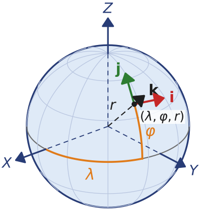
Global models use longitude \(\lambda\), latitude \(\varphi\) and the distance \(r\) from the centre of the Earth. Take Earth-fixed Cartesian axes \(X, Y, Z\), with \(Z\) along \(\boldsymbol{\Omega}\) and \(X\) towards longitude 0 (capitals, as \(z\) is the height above the surface, \(z = r - a\)). The position of a point is \[ \mathbf{r} = r\,(\cos\varphi\cos\lambda,\ \cos\varphi\sin\lambda,\ \sin\varphi) \] in these axes (Figure 21). Its derivatives along the coordinates give the local unit vectors east (\(\mathbf{i}\)), north (\(\mathbf{j}\)) and up (\(\mathbf{k}\)), each divided by its length: \[ \begin{aligned} \mathbf{i} &= \frac{1}{r\cos\varphi}\frac{\partial\mathbf{r}}{\partial\lambda} = (-\sin\lambda,\ \cos\lambda,\ 0),\\ \mathbf{j} &= \frac{1}{r}\frac{\partial\mathbf{r}}{\partial\varphi} = (-\sin\varphi\cos\lambda,\ -\sin\varphi\sin\lambda,\ \cos\varphi),\\ \mathbf{k} &= \frac{\partial\mathbf{r}}{\partial r} = (\cos\varphi\cos\lambda,\ \cos\varphi\sin\lambda,\ \sin\varphi) . \end{aligned} \] The lengths, \(r\cos\varphi\), \(r\) and 1, are the distances moved per unit change of each coordinate: a degree of longitude is shorter near the poles. Following a parcel, by the chain rule, \(D\mathbf{r}/Dt = r\cos\varphi\,(D\lambda/Dt)\,\mathbf{i} + r\,(D\varphi/Dt)\,\mathbf{j} + (Dr/Dt)\,\mathbf{k}\), so the velocity components are (Vallis 2017, sec. 2.2.2, eqs. 2.28–2.29) \[ u = r\cos\varphi\,\frac{D\lambda}{Dt}, \qquad v = r\,\frac{D\varphi}{Dt}, \qquad w = \frac{Dr}{Dt}, \qquad \mathbf{u} = u\,\mathbf{i} + v\,\mathbf{j} + w\,\mathbf{k} . \] The material derivative of a scalar is then (Vallis’s eq. 2.27) \[ \frac{D}{Dt} = \frac{\partial}{\partial t} + \frac{u}{r\cos\varphi}\frac{\partial}{\partial\lambda} + \frac{v}{r}\frac{\partial}{\partial\varphi} + w\frac{\partial}{\partial r} . \]
The unit vectors turn. Unlike Cartesian unit vectors, \(\mathbf{i}\), \(\mathbf{j}\), \(\mathbf{k}\) depend on position, so they change following a moving parcel. Differentiating them with respect to \(\lambda\) and \(\varphi\) (none depends on \(r\)), \(\partial\mathbf{i}/\partial\lambda = (-\cos\lambda, -\sin\lambda, 0) = \mathbf{j}\sin\varphi - \mathbf{k}\cos\varphi\), \(\partial\mathbf{j}/\partial\lambda = -\mathbf{i}\sin\varphi\), \(\partial\mathbf{j}/\partial\varphi = -\mathbf{k}\), \(\partial\mathbf{k}/\partial\lambda = \mathbf{i}\cos\varphi\), \(\partial\mathbf{k}/\partial\varphi = \mathbf{j}\), and using \(D\lambda/Dt = u/(r\cos\varphi)\) and \(D\varphi/Dt = v/r\): \[ \frac{D\mathbf{i}}{Dt} = \frac{u}{r\cos\varphi}\,(\mathbf{j}\sin\varphi - \mathbf{k}\cos\varphi), \qquad \frac{D\mathbf{j}}{Dt} = -\frac{u\tan\varphi}{r}\,\mathbf{i} - \frac{v}{r}\,\mathbf{k}, \qquad \frac{D\mathbf{k}}{Dt} = \frac{u}{r}\,\mathbf{i} + \frac{v}{r}\,\mathbf{j} . \tag{11}\] Vallis (2017, sec. 2.2.2, eqs. 2.36–2.39) obtains the same rates from the effective rotation of the axes as the parcel moves; here they come directly from the Cartesian components. The acceleration is therefore \[ \frac{D\mathbf{u}}{Dt} = \frac{Du}{Dt}\,\mathbf{i} + \frac{Dv}{Dt}\,\mathbf{j} + \frac{Dw}{Dt}\,\mathbf{k} + u\,\frac{D\mathbf{i}}{Dt} + v\,\frac{D\mathbf{j}}{Dt} + w\,\frac{D\mathbf{k}}{Dt} , \] and the last three terms give the metric terms (Section 27).
26 Spherical coordinates (2/3): grad, div, curl
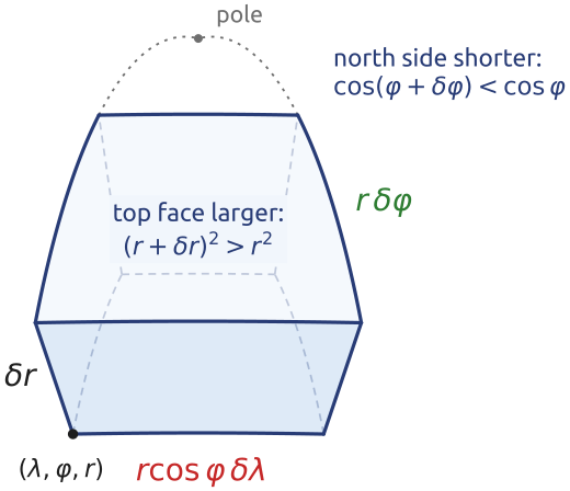
All the operators follow from a small grid box between \(\lambda\) and \(\lambda + \delta\lambda\), \(\varphi\) and \(\varphi + \delta\varphi\), \(r\) and \(r + \delta r\) (Figure 22): the box of the mass budget, on the sphere. Its edges have lengths \[ \delta x = r\cos\varphi\,\delta\lambda, \qquad \delta y = r\,\delta\varphi, \qquad \delta z = \delta r , \] and its volume is \(r^2\cos\varphi\,\delta\lambda\,\delta\varphi\,\delta r\). The areas of its faces change from one side to the other: the east and west faces have area \(r\,\delta\varphi\,\delta r\); the south and north faces \(r\cos\varphi\,\delta\lambda\,\delta r\), smaller on the north side, where the meridians converge; the bottom and top faces \(r^2\cos\varphi\,\delta\lambda\,\delta\varphi\), larger on top. The formulas below are those of Vallis (2017, sec. 2.2.2), derived here from the box.
Gradient (Vallis’s eq. 2.31): divide the change of a field along each edge by the edge’s length, \[ \nabla = \frac{\mathbf{i}}{r\cos\varphi}\frac{\partial}{\partial\lambda} + \frac{\mathbf{j}}{r}\frac{\partial}{\partial\varphi} + \mathbf{k}\,\frac{\partial}{\partial r} . \]
Divergence (eq. 2.30): the net flux of \(\mathbf{u} = u\,\mathbf{i} + v\,\mathbf{j} + w\,\mathbf{k}\) out of the box, divided by its volume. Through the east and west faces the area does not change with \(\lambda\), and the net outflow is \(\partial_\lambda u\,\delta\lambda\ r\,\delta\varphi\,\delta r\). Through the north and south faces the area changes with \(\varphi\), so \(\cos\varphi\) goes inside the derivative: \(\partial_\varphi(v\cos\varphi)\,\delta\varphi\ r\,\delta\lambda\,\delta r\). Through the top and bottom faces \(r^2\) goes inside: \(\partial_r(r^2 w)\,\delta r\ \cos\varphi\,\delta\lambda\,\delta\varphi\). Dividing by the volume, \[ \nabla\cdot\mathbf{u} = \frac{1}{r\cos\varphi}\frac{\partial u}{\partial\lambda} + \frac{1}{r\cos\varphi}\frac{\partial (v\cos\varphi)}{\partial\varphi} + \frac{1}{r^2}\frac{\partial (r^2 w)}{\partial r} . \] The continuity equation in flux form is then (Vallis 2017, eq. 2.41) \[ \frac{\partial\rho}{\partial t} + \frac{1}{r\cos\varphi}\frac{\partial(\rho u)}{\partial\lambda} + \frac{1}{r\cos\varphi}\frac{\partial(\rho v\cos\varphi)}{\partial\varphi} + \frac{1}{r^2}\frac{\partial(r^2\rho w)}{\partial r} = 0 . \]
Vorticity. The circulation round the top face, divided by its area (Stokes’s theorem), is the vertical component of the curl. Going round the face anticlockwise seen from above, the circulation gains \((u\cos\varphi)\big|_{\varphi}\,r\,\delta\lambda\) along the south edge (of length \(r\cos\varphi\,\delta\lambda\)) and loses \((u\cos\varphi)\big|_{\varphi+\delta\varphi}\,r\,\delta\lambda\) along the north edge; it gains \(v\big|_{\lambda+\delta\lambda}\,r\,\delta\varphi\) along the east edge and loses \(v\big|_{\lambda}\,r\,\delta\varphi\) along the west edge (both of length \(r\,\delta\varphi\)). The circulation is \(r\,\delta\lambda\,\delta\varphi\,[\partial_\lambda v - \partial_\varphi(u\cos\varphi)]\), and dividing by the area \(r^2\cos\varphi\,\delta\lambda\,\delta\varphi\), \[ \zeta = \mathbf{k}\cdot\nabla\times\mathbf{u} = \frac{1}{r\cos\varphi}\Big[\frac{\partial v}{\partial\lambda} - \frac{\partial (u\cos\varphi)}{\partial\varphi}\Big], \] the spin of the flow about the local vertical. The other faces give the other components; the full curl (Vallis’s eq. 2.33, written there as a determinant) is \[ \nabla\times\mathbf{u} = \frac{\mathbf{i}}{r}\Big[\frac{\partial w}{\partial\varphi} - \frac{\partial (r v)}{\partial r}\Big] + \frac{\mathbf{j}}{r}\Big[\frac{\partial (r u)}{\partial r} - \frac{1}{\cos\varphi}\frac{\partial w}{\partial\lambda}\Big] + \frac{\mathbf{k}}{r\cos\varphi}\Big[\frac{\partial v}{\partial\lambda} - \frac{\partial (u\cos\varphi)}{\partial\varphi}\Big] . \]
Laplacian (eq. 2.32): the divergence of the gradient, \(\nabla^2 = \nabla\cdot\nabla\), \[ \nabla^2 = \frac{1}{r^2\cos^2\varphi}\frac{\partial^2}{\partial\lambda^2} + \frac{1}{r^2\cos\varphi}\frac{\partial}{\partial\varphi}\Big(\cos\varphi\,\frac{\partial}{\partial\varphi}\Big) + \frac{1}{r^2}\frac{\partial}{\partial r}\Big(r^2\frac{\partial}{\partial r}\Big) . \] The Laplacian of a vector (for the viscous term \(\nu\nabla^2\mathbf{u}\)) is not this operator applied to each component, because the unit vectors change with position; it follows from \(\nabla^2\mathbf{u} = \nabla(\nabla\cdot\mathbf{u}) - \nabla\times(\nabla\times\mathbf{u})\) (Vallis’s eq. 2.34).
27 Spherical coordinates (3/3): momentum
Metric terms. With Equation 11, the last three terms of the acceleration are \[ u\,\frac{D\mathbf{i}}{Dt} + v\,\frac{D\mathbf{j}}{Dt} + w\,\frac{D\mathbf{k}}{Dt} = \mathbf{i}\Big(- \frac{uv\tan\varphi}{r} + \frac{uw}{r}\Big) + \mathbf{j}\Big(\frac{u^2\tan\varphi}{r} + \frac{vw}{r}\Big) - \mathbf{k}\,\frac{u^2 + v^2}{r} \] (Vallis 2017, eq. 2.45). These are the metric terms: a parcel moving east at constant speed along a latitude circle does not move in a straight line, and its acceleration towards the axis appears in the \(\mathbf{j}\) and \(\mathbf{k}\) components.
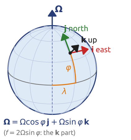
Coriolis terms. At latitude \(\varphi\) the rotation vector is \(\boldsymbol{\Omega} = \Omega\cos\varphi\,\mathbf{j} + \Omega\sin\varphi\,\mathbf{k}\) (Figure 23), so (Vallis’s eqs. 2.36 and 2.46) \[ 2\boldsymbol{\Omega}\times\mathbf{u} = (2\Omega w\cos\varphi - 2\Omega v\sin\varphi)\,\mathbf{i} + 2\Omega u\sin\varphi\,\mathbf{j} - 2\Omega u\cos\varphi\,\mathbf{k} . \] Its vertical part, \(\Omega\sin\varphi\), gives the Coriolis parameter \(f = 2\Omega\sin\varphi\).
The result. With the geopotential surfaces taken as spheres, \(\Phi = gz\) with \(z = r - a\), the three components of Equation 10 without friction are (Vallis 2017, sec. 2.2.3, eqs. 2.47a–c; Holton 2004, sec. 2.3) \[ \begin{aligned} \frac{Du}{Dt} - \Big(2\Omega + \frac{u}{r\cos\varphi}\Big)(v\sin\varphi - w\cos\varphi) &= -\frac{1}{\rho\,r\cos\varphi}\frac{\partial p}{\partial\lambda},\\ \frac{Dv}{Dt} + \frac{wv}{r} + \Big(2\Omega + \frac{u}{r\cos\varphi}\Big)u\sin\varphi &= -\frac{1}{\rho\,r}\frac{\partial p}{\partial\varphi},\\ \frac{Dw}{Dt} - \frac{u^2 + v^2}{r} - 2\Omega u\cos\varphi &= -\frac{1}{\rho}\frac{\partial p}{\partial r} - g , \end{aligned} \tag{12}\] with the material derivative of a scalar for \(D/Dt\); friction adds its components to the right-hand sides. Vallis calls the terms with \(\Omega\) the Coriolis terms, and the quadratic terms with \(1/r\) the metric terms. Richardson (1922) wrote these equations for his forecast by hand (Richardson 1922).
The metric and Coriolis terms combine: \(\Omega + u/(r\cos\varphi)\) is the rate at which a parcel turns about the axis seen from space. Without an east–west force the first equation keeps the angular momentum per unit mass about the axis, \(m = (\Omega r\cos\varphi + u)\,r\cos\varphi\): since \(D(r\cos\varphi)/Dt = w\cos\varphi - v\sin\varphi\), \[ \frac{Dm}{Dt} = r\cos\varphi\,\Big[\frac{Du}{Dt} - \Big(2\Omega + \frac{u}{r\cos\varphi}\Big)(v\sin\varphi - w\cos\varphi)\Big] = -\frac{1}{\rho}\frac{\partial p}{\partial\lambda} . \]
Thin layers. The atmosphere and the ocean are thin compared with the Earth’s radius. Two approximations go together (Vallis 2017, sec. 2.2.4): the shallow-fluid approximation, \(r\) replaced by \(a\) except where it is differentiated (\(r = a + z\)); and the traditional approximation, which drops the Coriolis terms with \(\Omega\cos\varphi\) in the horizontal equations and the metric terms \(uw/r\) and \(vw/r\). They “should be taken, or not, together”: both rest on the small aspect ratio of the motion, and with one but not the other, angular momentum and energy are no longer conserved. Taken together, the horizontal equations become (Vallis’s eqs. 2.50a,b) \[ \frac{Du}{Dt} - f v - \frac{uv\tan\varphi}{a} = -\frac{1}{\rho\,a\cos\varphi}\frac{\partial p}{\partial\lambda}, \qquad \frac{Dv}{Dt} + f u + \frac{u^2\tan\varphi}{a} = -\frac{1}{\rho\,a}\frac{\partial p}{\partial\varphi}, \] and the angular momentum \(m = (\Omega a\cos\varphi + u)\,a\cos\varphi\) is kept again. With a third approximation, hydrostatic balance in the vertical, \(\partial p/\partial z = -\rho g\) (which also drops \(2\Omega u\cos\varphi\) and \((u^2 + v^2)/r\) from the vertical equation), they form the primitive equations (Vallis’s eqs. 2.50a–c).
28 Thermodynamics (1/5): the gas law
Dry air is very nearly an ideal gas (Vallis 2017, sec. 1.4, eq. 1.53): \[ p = \rho R T , \] with \(T\) in kelvin and the gas constant of dry air \(R = R^*/M = 8.314/0.029 \approx 287\) J/(kg K), where \(R^* = 8.314\) J/(mol K) is the universal gas constant and \(M = 0.029\) kg/mol the mean molar mass of dry air (Vallis writes \(\mu\) for it; here \(\mu\) is the dynamic viscosity). It is a fifth equation, but it adds a sixth unknown, \(T\): density follows from pressure and temperature, and knowing two of \(p\), \(\rho\), \(T\) gives the third. Water vapour, lighter than dry air, changes the gas constant slightly: with specific humidity \(q\), \(p = \rho R T\,(1 + 0.608\,q)\) (Cushman-Roisin and Beckers 2011, sec. 3.3, eq. 3.6).
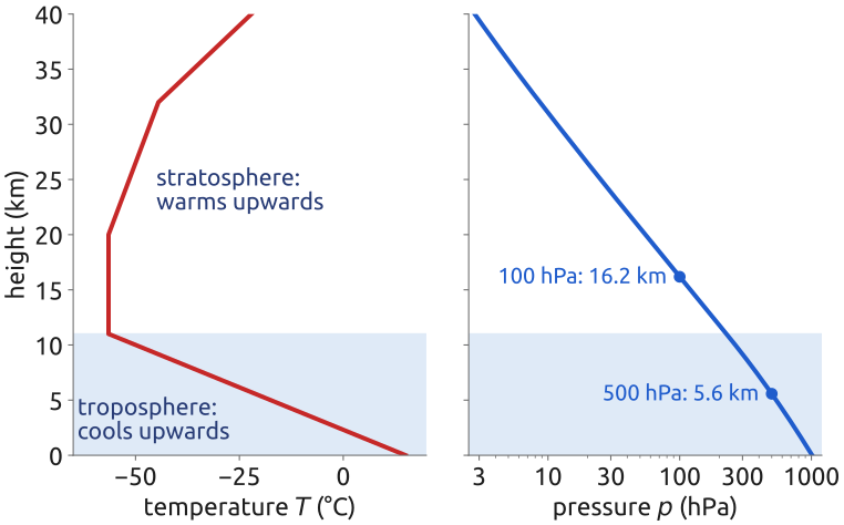
The U.S. Standard Atmosphere (Figure 24) is a formula, not an observation: it prescribes the temperature as piecewise linear in height (falling by 6.5 K/km from 288.15 K at sea level to 11 km, constant to 20 km, then rising) and gets the pressure by integrating the hydrostatic balance \(\partial p/\partial z = -\rho g\) with the gas law (NOAA et al. 1976). The pressure falls nearly exponentially, halving about every 5.5 km: 500 hPa at 5.6 km, 100 hPa at 16.2 km.
29 Thermodynamics (2/5): the first law
Per unit mass, the heat added to a parcel goes into its internal energy and into the work it does in expanding against its surroundings. For an ideal gas the internal energy is \(c_v T\), and the work done when the specific volume \(\alpha = 1/\rho\) grows by \(d\alpha\) is \(p\,d\alpha\). Following a parcel, \[ Q = c_v\frac{DT}{Dt} + p\,\frac{D\alpha}{Dt} , \] with \(Q\) the heating rate per unit mass (radiation, release of latent heat, conduction), in W/kg, and \(c_v = 717\) J/(kg K) the specific heat at constant volume. By mass continuity, Equation 4, \(D\alpha/Dt = \alpha\,\nabla\cdot\mathbf{u}\): the work is done by the expansion of the parcel, and the law reads \(c_v\,DT/Dt + p\alpha\nabla\cdot\mathbf{u} = Q\) (Vallis 2017, sec. 1.6.1, eq. 1.100). Differentiating the gas law \(p\alpha = RT\) gives \(p\,D\alpha/Dt = R\,DT/Dt - \alpha\,Dp/Dt\), and with \(c_p = c_v + R\): \[ c_p\frac{DT}{Dt} - \frac{1}{\rho}\frac{Dp}{Dt} = Q , \tag{13}\] with \(c_p = 1004\) J/(kg K), the specific heat of dry air at constant pressure (Vallis 2017, sec. 1.6.1; Holton 2004, sec. 2.6).
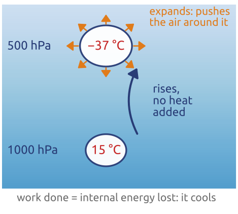
Adiabatic means \(Q = 0\): no heat exchanged. It does not mean constant temperature. A parcel that rises without exchanging heat finds a lower pressure, expands, does work on its surroundings and cools (Figure 25): with \(Q = 0\), \(c_p\,dT = dp/\rho\), and integrating with the gas law gives \(T = T_0\,(p/p_0)^{R/c_p}\), from \(15\,^\circ\)C at 1000 hPa to about \(-37\,^\circ\)C at 500 hPa. Rising air cools until its water vapour condenses and clouds form; from then on the latent heat released makes \(Q > 0\).
30 Thermodynamics (3/5): potential temperature
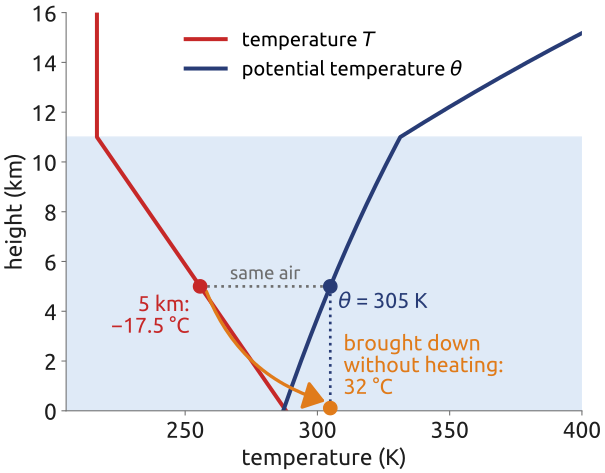
Definition. The potential temperature \(\theta\) of a parcel is the temperature it would have if moved adiabatically (\(Q = 0\)) to the reference pressure \(p_0 = 1000\) hPa (Vallis 2017, sec. 1.6.1, who writes \(p_R\)). The move is imagined: it serves only to define \(\theta\). On the way, the first law with \(Q = 0\), divided by \(T\), and the gas law in the form \(1/(\rho T) = R/p\) give \[ c_p\,d\ln T = R\,d\ln p . \] Integrating along the move, from \((T, p)\) to \((\theta, p_0)\) (Vallis’s eqs. 1.103–1.104), \[ \int_T^{\theta} c_p\,d\ln T - \int_p^{p_0} R\,d\ln p = 0 \quad\Rightarrow\quad \ln\frac{\theta}{T} = \frac{R}{c_p}\,\ln\frac{p_0}{p} , \] for constant \(c_p\) and \(R\), so that (Vallis’s eq. 1.105, with \(\kappa = R/c_p\)) \[ \theta = T\left(\frac{p_0}{p}\right)^{R/c_p}, \qquad R/c_p = 0.286 \text{ for dry air.} \tag{14}\] It is a function of \(T\) and \(p\) alone: every parcel has a \(\theta\), wherever it is. \(\theta\) takes out the cooling by expansion. In the standard atmosphere \(T = 255.7\) K (\(-17.5\,^\circ\)C) at 5 km, where \(p = 540\) hPa, so \(\theta = 304.9\) K: brought down to the ground without heating, that air would arrive at about \(32\,^\circ\)C, as in a foehn wind (Figure 26). Potential temperature grows with height (by about 3 to 5 K/km in the standard troposphere, much faster in the stratosphere): a parcel pushed up keeps its \(\theta\), finds itself colder and denser than its new surroundings, and sinks back. The atmosphere is stably stratified (Holton 2004, sec. 2.7).
31 Thermodynamics (4/5): how \(\theta\) changes
Now follow the real flow, with any heating \(Q\). Take the logarithm of Equation 14 and its material derivative: \[ \begin{aligned} \ln\theta &= \ln T - \frac{R}{c_p}\ln p + \text{const},\\ c_p\frac{D\ln\theta}{Dt} &= \frac{c_p}{T}\frac{DT}{Dt} - \frac{R}{p}\frac{Dp}{Dt}\\ &= \frac{1}{T}\left(c_p\frac{DT}{Dt} - \frac{1}{\rho}\frac{Dp}{Dt}\right) && \text{(gas law: } R/p = 1/(\rho T))\\ &= \frac{Q}{T} && \text{(first law)} . \end{aligned} \] With \(D\ln\theta/Dt = (1/\theta)\,D\theta/Dt\), the thermodynamic equation in terms of \(\theta\) (Vallis 2017, sec. 1.6.1, eqs. 1.106–1.108; Holton 2004, sec. 2.7): \[ \frac{D\theta}{Dt} = \frac{\theta}{c_p T}\,Q . \tag{15}\] In adiabatic flow, \(Q = 0\), \(D\theta/Dt = 0\): \(\theta\) is kept, carried by each parcel like a label. Heating raises \(\theta\), cooling lowers it. \(Q = 0\) is used twice, with two meanings: an imagined adiabatic move defines \(\theta\); a real adiabatic flow keeps it.
\(\theta\) is a measure of entropy: per unit mass, \(d\eta = c_p\,d\ln\theta\), so \(\eta = c_p\ln\theta\) up to a constant (Vallis’s eqs. 1.106–1.107, \(\eta\) the specific entropy), and adiabatic flow is isentropic. Because \(\theta\) is a label carried by the parcels in adiabatic flow, surfaces of constant \(\theta\) are then material surfaces, the basis of isentropic analysis and of potential vorticity (Vallis 2017, Ch. 4).
32 Thermodynamics (5/5): seawater
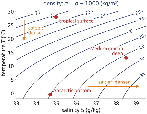
Seawater is a solution of salts, about 35 g of salt per kg of seawater; the mass fraction of salt, in g/kg, is the salinity \(S\). Its density depends on temperature, salinity and pressure, \(\rho = \rho(T, S, p)\), through an empirical formula: the present standard is TEOS-10, the International Thermodynamic Equation of Seawater (IOC et al. 2010; Vallis 2017, sec. 1.4 and §1.7.2). Near a reference state \((T_0, S_0)\), and leaving out the effect of pressure (it changes the density a lot, but mostly in the vertical, where it is balanced by the weight of the water: the horizontal differences that drive currents come from temperature and salinity (Vallis 2017, sec. 1.4)), a linear equation of state is often enough for understanding: \[ \rho = \rho_0\big[1 - \beta_T(T - T_0) + \beta_S(S - S_0)\big], \] with typical values \(\rho_0 = 1028\) kg/m\(^3\), \(T_0 = 10\,^\circ\)C, \(S_0 = 35\) g/kg, \(\beta_T = 1.7\times10^{-4}\) K\(^{-1}\) (the thermal expansion coefficient) and \(\beta_S = 7.6\times10^{-4}\) (g/kg)\(^{-1}\) (the haline contraction coefficient), in the notation of Vallis (2017, sec. 1.4, eq. 1.57) (values from Cushman-Roisin and Beckers 2011, sec. 3.3, eq. 3.4, who writes \(\alpha\) and \(\beta\)). Warmer water is lighter, saltier water denser. The coefficients are not constant: \(\beta_T\) is much smaller in cold water than in warm water, which curves the contours of Figure 27 (Vallis’s simplified nonlinear equation of state, his eq. 1.58 with Table 1.2) and has consequences such as cabbeling: two waters of the same density, mixed, give a denser water. Seawater hardly compresses: a parcel moved adiabatically from the surface to 5 km depth becomes only about 2.5 % denser (Vallis 2017, sec. 1.6.2).
Heat and salt. Salt is carried by the water and changes only by non-conservative effects (Vallis 2017, sec. 1.6, eq. 1.96): \[ \frac{DS}{Dt} = \dot S , \] with \(\dot S\) from evaporation (which concentrates the salt) and rain, rivers and melting ice (which dilute it) at the surface, and from mixing inside the ocean. For the heat, the variable is the potential temperature of seawater, \(\theta\): the temperature a parcel would have if moved adiabatically to the surface pressure. As for air (Vallis 2017, sec. 1.7.1, eq. 1.141), \[ c_p\frac{D\theta}{Dt} = \frac{\theta}{T}\,Q, \qquad\text{that is}\qquad \frac{D\theta}{Dt} = \dot\theta , \] with \(c_p \approx 4000\) J/(kg K) for seawater (3986 in Vallis’s Table 1.2) and the sources \(\dot\theta\), heating and cooling by the atmosphere and the Sun, at the surface, and mixing inside. In-situ temperature \(T\) is not kept in adiabatic motion: compression warms a sinking parcel, by about 0.15 K/km, the adiabatic lapse rate \(\Gamma = g\beta_T T/c_p\) (Vallis 2017, sec. 1.6.2, eqs. 1.124–1.130). (TEOS-10 uses conservative temperature, very close to \(\theta\), as its heat variable (Vallis 2017, sec. 1.7.3).)
33 In class: Gibraltar and the deep water
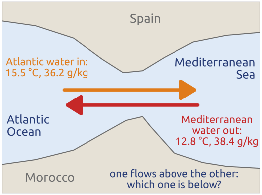
Exercise 2 — Who wins, temperature or salinity? Use the linear equation of state \(\rho = \rho_0\,[1 - \beta_T (T - T_0) + \beta_S (S - S_0)]\) with \(\rho_0 = 1028\) kg/m\(^3\), \(\beta_T = 1.7\times10^{-4}\) K\(^{-1}\), \(\beta_S = 7.6\times10^{-4}\) (g/kg)\(^{-1}\). At Gibraltar, Atlantic water flows into the Mediterranean (15.5 \(^\circ\)C, \(S = 36.2\) g/kg) and Mediterranean water flows out (12.8 \(^\circ\)C, \(S = 38.4\) g/kg). (a) Which water is denser, by how many kg/m\(^3\)? Which one flows out at the bottom? (b) Which difference matters more, temperature or salinity? How warm would the Mediterranean water have to be to flow out on top?
(c) Where does deep water form? Compare warm, salty subtropical surface water (25 \(^\circ\)C, \(S = 37.0\) g/kg) with cold, fresher Labrador Sea water in winter (3 \(^\circ\)C, \(S = 34.9\) g/kg). Which is denser, by how much, and which difference wins here? Where in the ocean would you expect water to sink to the bottom?
The setting is in Figure 28; the data come from Cushman-Roisin and Beckers (2011, sec. 3.3 and problem 3.4).
34 The equations of motion, derived
Collecting the results, for the atmosphere: \[ \begin{aligned} &\frac{D\mathbf{u}}{Dt} + 2\boldsymbol{\Omega}\times\mathbf{u} = -\frac{1}{\rho}\nabla p - \nabla\Phi + \mathbf{F} && \text{(3 equations)}\\ &\frac{D\rho}{Dt} + \rho\,\nabla\cdot\mathbf{u} = 0 && \text{(1)}\\ &p = \rho R T && \text{(1)}\\ &c_p\frac{DT}{Dt} - \frac{1}{\rho}\frac{Dp}{Dt} = Q && \text{(1)}\\ &\frac{Dq}{Dt} = \dot q && \text{(1)} \end{aligned} \] seven equations for the seven unknowns \(u, v, w, p, \rho, T, q\), as Bjerknes counted (Bjerknes 1904; Cushman-Roisin and Beckers 2011, sec. 3.6). Each term has its derivation: the acceleration is the material derivative of a parcel’s velocity; the Coriolis term comes from the rotating frame; the pressure force from the pressures on the faces of a box; \(-\nabla\Phi\) is gravity plus the centrifugal force; \(\mathbf{F}\) is friction (molecular viscosity \(\nu\nabla^2\mathbf{u}\), in practice turbulence, parameterized); mass continuity comes from the box or the moving parcel; then the gas law and the first law.
The seventh equation carries the water vapour. The specific humidity \(q\) is carried by the air, with sources and sinks \(\dot q\): evaporation at the surface and from falling rain, condensation in clouds (Vallis 2017, sec. 1.6.1, eq. 1.102). Condensation releases latent heat, about 2.5 MJ per kg of water, which enters the heating: \(Q = -L\dot q\) for condensation, with \(L\) the latent heat. The moisture and heat equations are therefore coupled, and clouds and rain are among the hardest parts of a model.
For the ocean the salinity \(S\) takes the place of \(q\), with \(DS/Dt = \dot S\); the equation of state of seawater, \(\rho = \rho(T, S, p)\), takes the place of the gas law; and the heat equation of seawater, \(D\theta/Dt = \dot\theta\), takes the place of the first law of an ideal gas (Cushman-Roisin and Beckers 2011, sec. 3.6; Vallis 2017, sec. 1.7). With boundary conditions (no flow through the ground and the sea floor; fluxes of heat, water and momentum at the surface) and the forcing terms \(\mathbf{F}\), \(Q\), \(\dot q\), \(\dot S\), \(\dot\theta\) (the “physics” of the models), this is the closed system that weather, ocean and climate models start from. On the sphere the momentum equation is written as in Equation 12.
35 Fast and slow: what the equations allow
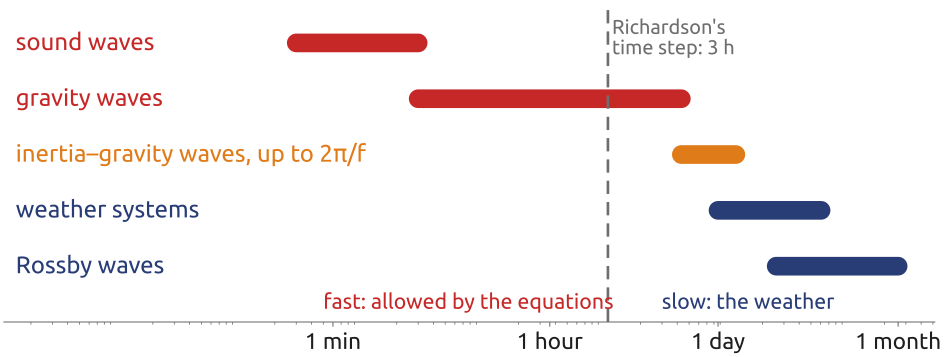
The closed system holds more than the weather. Three restoring mechanisms give it fast waves (Figure 29):
- Sound waves, from compressibility: a compressed parcel pushes back. In air the speed is \(c_s = \sqrt{\gamma R T} \approx 340\) m/s, with \(\gamma = c_p/c_v = 1.4\); in seawater about 1500 m/s (Vallis 2017, sec. 1.8). Sound crosses 100 km in 5 minutes.
- Gravity waves, from buoyancy and the free surface: a displaced parcel or a raised sea surface falls back and overshoots. The fastest, involving the whole depth of the fluid, travel at \(\sqrt{gH}\) (\(H\): the depth): about 200 m/s in the deep ocean and about 300 m/s in the atmosphere. Internal gravity waves are slower, with periods from the buoyancy period \(2\pi/N\), about 10 minutes (\(N \approx 0.01\) s\(^{-1}\), the buoyancy frequency), to hours (Vallis 2017, Ch. 7).
- Inertia–gravity waves, gravity waves feeling the rotation: their frequencies lie between \(f\) and \(N\), so their longest periods reach the inertial period \(2\pi/f\), 12 h at the poles and 17 h at Milan (Vallis 2017, sec. 3.8 and §7.6, eq. 7.127). In the limit of horizontal motion they are the inertial oscillations of Section 23.
The weather systems we forecast are much slower: a cyclone 1000 km across, moving at 10 m/s, passes in about a day and lives about a week; planetary (Rossby) waves take days to a month.
The fast waves matter for computing. Richardson (1922) computed by hand the six-hour change of pressure from observed winds and pressures, with the hydrostatic primitive equations, which have no vertically travelling sound waves but still carry gravity waves. The observations were slightly out of balance and excited them: he found “145 millibars in 6 hours, whereas observations show that the barometer was nearly steady” (Richardson 1922, 187; Lynch 1999, 2008). His three-hour time step would also have been too long for these waves had he gone on: a time step must not let the fastest wave cross more than about one grid interval (Courant et al. 1928; Vallis 2017, Ch. 11, note 4, p. 442). Models either take short steps, treat the fast waves implicitly, or filter them out of the equations by scale analysis.
36 Key points
- \(D/Dt = \partial/\partial t + \mathbf{u}\cdot\nabla\): the rate of change following a parcel, against the change at a fixed point; advection links them.
- Mass: \(\partial_t\rho + \nabla\cdot(\rho\mathbf{u}) = 0\) for a box fixed in space, equivalent to \(D\rho/Dt = -\rho\,\nabla\cdot\mathbf{u}\) for a parcel; \(\nabla\cdot\mathbf{u}\) is the rate at which a parcel’s volume grows.
- Momentum on the rotating Earth: \(D\mathbf{u}/Dt + 2\boldsymbol{\Omega}\times\mathbf{u} = -\nabla p/\rho - \nabla\Phi + \mathbf{F}\); the Coriolis term has two equal halves; the centrifugal force is kept inside \(\Phi\), and \(\Phi \approx gz\) is a small geometric approximation.
- Heat: \(\theta = T(p_0/p)^{R/c_p}\) is kept in adiabatic motion; seawater: \(\rho(T, S, p)\), with heat (\(\theta\)) and salt carried by the water.
- Seven equations for seven unknowns, for air and for seawater; they allow fast waves, sound and gravity waves (with rotation, inertia–gravity waves), besides the slow weather.
Further reading
Vallis (2017), Ch. 1 and §2.1–2.2, for everything in these notes; Cushman-Roisin and Beckers (2011), Ch. 2 (the Coriolis force, with numerical methods for oscillations) and Ch. 3 (the equations); Holton (2004), Ch. 1–2, for an intuitive derivation; Zdunkowski and Bott (2003) for complete derivations, including general curvilinear coordinates; Persson (1998) and Durran (1993) on how to understand the Coriolis force; Chorin and Marsden (1993) for the mathematical theory.