November 2026 · Politecnico di Milano

The equations of motion from basic principles

Atmosphere and Ocean Dynamics — Lecture 2

Prof. Dr. Pedro da Silva Peixoto

Applied Mathematics
Instituto de Matemática e Estatística
Universidade de São Paulo

Visiting Professor at MOX Lab
Politecnico di Milano

Warm-up

1. What is the Coriolis parameter \(f\) at Milan (\(45.5^\circ\)N)? What is its sign in Sydney?
2. In Milan you stand with the wind at your back: where is the low pressure? Why does the wind not blow from high to low pressure?
3. A sea breeze (5 m/s, 20 km) and a cyclone (10 m/s, 1000 km): which one feels the Earth’s rotation?
4. Bjerknes (1904): what two things does a forecast need?

Lecture 1, from memory: answer on paper first, 3 minutes (its carry-forward list).

1. f = 2 Omega sin(lat) = 1.04e-4 1/s; negative in the south (Sydney 34S: -0.8e-4).
2. On your left; the Coriolis force balances the pressure force: geostrophic wind.
3. Ro = U/(fL): sea breeze 2.4, cyclone 0.1: the cyclone.
4. The state now, and the laws: today we derive the laws.

Where we are and where we are going

Previous knowledge

• Vector calculus (gradient, divergence, the divergence (Gauss’s) theorem), Taylor series, Newton’s second law
• Rotation: \(f = 2\Omega\sin\varphi\) (\(1.04\times10^{-4}\ \mathrm{s^{-1}}\) at Milan) turns moving air and water to the right in the northern hemisphere; geostrophic wind along the isobars when \(Ro = U/(fL) \ll 1\)
• A forecast is an initial-value problem: the state now, and the laws (Bjerknes, 1904)
• The laws, as a box of equations: Euler’s equations (with friction: Navier–Stokes), the Coriolis term, the gas law, the first law

Where we are going

1. Fluid parcels and the material derivative
2. Mass: a box fixed in space, then a moving parcel
3. Momentum: pressure, gravity, friction
4. The rotating frame: Coriolis, geopotential, notebook
5. Spherical coordinates: the equations on the sphere
6. Heat: gas law, first law, potential temperature, seawater
7. Seven equations, seven unknowns, and their waves

Newton’s laws for a fluid on the rotating Earth, term by term

(Vallis 2017, Ch. 1–2; Cushman-Roisin and Beckers 2011, Ch. 2–3)

Two minutes. Left: what we take as known (the warm-up checked it). Right: the road of the day; each item links to its first slide.

The equations of motion

\[\underbrace{\frac{D\mathbf{u}}{Dt}}_{\text{Newton, Euler}} + \underbrace{2\boldsymbol{\Omega}\times\mathbf{u}}_{\text{Coriolis}} = \underbrace{-\frac{1}{\rho}\nabla p}_{\text{Euler, Torricelli}} \underbrace{-\,\nabla\Phi}_{\text{gravity}} + \underbrace{\nu\nabla^2\mathbf{u}}_{\text{Navier, Stokes}}\]

\[\underbrace{\frac{D\rho}{Dt} + \rho\,\nabla\cdot\mathbf{u} = 0}_{\text{continuity (Euler)}} \qquad \underbrace{p = \rho R T}_{\text{ideal gas law}}, \quad \underbrace{c_p\frac{DT}{Dt} - \frac{1}{\rho}\frac{Dp}{Dt} = Q}_{\text{first law}} \qquad \underbrace{\frac{Dq}{Dt} = \dot q}_{\text{water vapour}}\]

\(\mathbf{u} = (u, v, w)\): velocity; \(D/Dt\): rate of change following the fluid; \(\boldsymbol{\Omega}\): Earth’s rotation; \(\rho\): density; \(p\): pressure; \(\Phi\): geopotential; \(\nu\): viscosity; \(T\): temperature; \(c_p\): specific heat; \(R\): gas constant; \(Q\): heating; \(q\): water vapour; \(\dot q\): its sources (the dot names a source, not a time derivative)

• Seven unknowns \(u, v, w, p, \rho, T, q\); seven equations: Bjerknes’ programme (1904)
• The ocean: salinity instead of water vapour, and the equation of state of seawater

Today: each term derived for a fluid on the rotating Earth

(Bjerknes 1904; Vallis 2017, Ch. 1)

Today we derive these equations term by term; at the end the same box comes back with the derivation under each term. D/Dt: following the parcel. Phi: gravity plus the centrifugal force. Next: Newton’s laws are for bodies; what is a “body” in a fluid that flows and deforms?

Fluid parcels

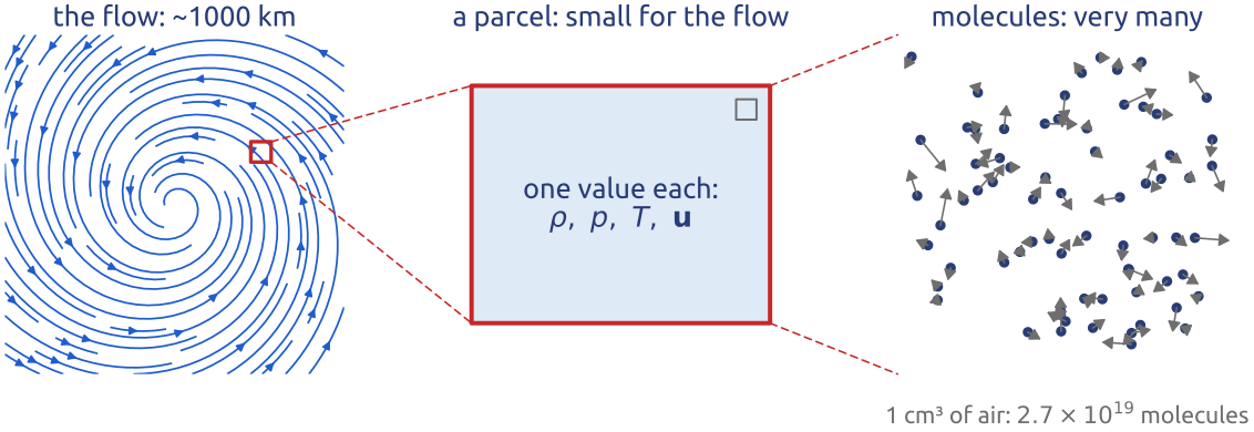
• A parcel: small compared with the flow, so it has one density, pressure, temperature, velocity

• Large compared with the molecules: the fluid is a continuum, and \(\rho\), \(p\), \(T\), \(\mathbf{u}\) are smooth fields of \((\mathbf{x}, t)\)

Newton’s laws apply to each parcel; but parcels move: follow them, or watch a fixed place?

(Vallis 2017, sec. 1.1; Holton 2004, sec. 1.1)

1 cm3 of air at sea level (15 C): 2.5e19 molecules; mean free path 0.07 micrometres. A parcel can be 1 m or 1 km: small for a 1000 km cyclone. The continuum hypothesis fails only in the upper atmosphere.

Two views: Lagrangian and Eulerian

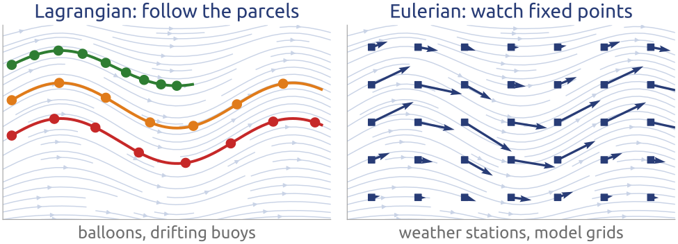
• Lagrangian: follow each parcel, \(\mathbf{x}(t)\), \(T(t)\)

• Eulerian: fields at fixed points, \(T(\mathbf{x}, t)\), \(\mathbf{u}(\mathbf{x}, t)\)

Physical laws are simplest for parcels; measurements and models are mostly on fixed grids

(Vallis 2017, sec. 1.1.1; Cushman-Roisin and Beckers 2011, Ch. 3)

Ask first: at night a weather station sees the temperature drop by 2 K in an hour. Did every parcel of air over it cool by 2 K? (Not necessarily: colder air may be blowing in.) Lagrange and Euler both used both views; the names are conventional.

Material derivative (1/2): follow the parcel

A parcel at \(\mathbf{x}\) at time \(t\) is at \(\mathbf{x} + \mathbf{u}\,\delta t\) at \(t + \delta t\). The change of \(T\) it feels (Taylor, to first order in \(\delta t\)):

\[\begin{aligned} \delta T &= T(\mathbf{x} + \mathbf{u}\,\delta t,\ t + \delta t) - T(\mathbf{x}, t)\\ &\approx \frac{\partial T}{\partial t}\,\delta t + {\color{#1f5ccc}{u\frac{\partial T}{\partial x}\delta t + v\frac{\partial T}{\partial y}\delta t + w\frac{\partial T}{\partial z}\delta t}} \end{aligned}\]

Divide by \(\delta t\), let \(\delta t \to 0\): the rate of change following the parcel.

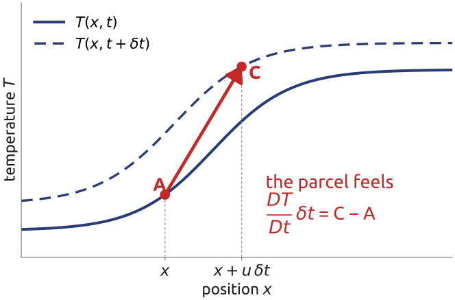
A parcel’s temperature changes because the field changes in time and because the parcel moves

(Vallis 2017, sec. 1.1.2; Holton 2004, sec. 2.1)

Board: Taylor expansion to first order in dt. The blue terms: moving through a field that varies in space. One dimension in the figure, three on the board.

Material derivative (2/2): change and advection

\[\frac{DT}{Dt} = \underbrace{\frac{\partial T}{\partial t}}_{\text{at a fixed point}} + \underbrace{{\color{#1f5ccc}{\mathbf{u}\cdot\nabla T}}}_{\text{advection}}\]

• \(D/Dt = \partial_t + \mathbf{u}\cdot\nabla\): the material derivative, for any field
• If the parcels keep their temperature, \(DT/Dt = 0\): a fixed station sees \(\partial T/\partial t = -\mathbf{u}\cdot\nabla T\)
• Acceleration of a parcel: \(D\mathbf{u}/Dt\), nonlinear in \(\mathbf{u}\)

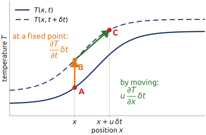
Laws hold for parcels (\(D/Dt\)); models compute at fixed points (\(\partial/\partial t\)): advection links them

(Vallis 2017, sec. 1.1.2; Cushman-Roisin and Beckers 2011, sec. 3.2)

A to C splits into A to B (field changes at x) and B to C (moving along the new profile). u . grad u: the nonlinearity of fluid dynamics; advection schemes are lecture 5.

In class: a thermometer in the wind

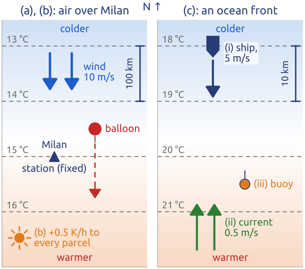
Exercise 1 — Eulerian and Lagrangian. A wind of 10 m/s blows southward over Milan; the air is colder towards the north: the temperature falls by 1 K every 100 km. (a) If each parcel keeps its temperature, how fast does the thermometer of a weather station in Milan change (K/h)? (b) The Sun now warms every parcel by 0.5 K/h. What does the station record? And a balloon drifting with the air?

Southward wind: \(v = -10\) m/s. Colder to the north: \(\partial T/\partial y < 0\).

(c) A ship crossing a front. A research ship sails south at 5 m/s across an ocean front where the surface water warms by 1 K every 10 km towards the south. (i) The front does not move and there is no current: what does the ship’s thermometer record (K/h)? (ii) The ship stops; a current of 0.5 m/s flows north and carries the water with its temperature: what does it record now? (iii) And a buoy drifting with the current? Which time derivative is each one?

In notebook 02a (exercise 1.1): open in Colab · download

(Vallis 2017, sec. 1.1)

1. dT/dt = -v dT/dy = -(-10)(-1e-5) = -1e-4 K/s = -0.36 K/h: the station cools.
2. station: 0.5 - 0.36 = +0.14 K/h; balloon: DT/Dt = +0.5 K/h.
3. ship (its own path): +1.8 K/h; stopped ship: +0.18 K/h (warm water arrives from the south); buoy: 0. Three derivatives: along a path, at a point, following the fluid.

Mass (1/4): a box fixed in space

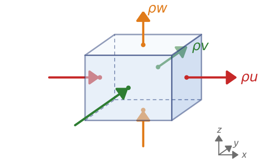
A small box, edges \(\delta x, \delta y, \delta z\), fixed in space (a control volume). The mass inside:

\[\begin{aligned}M &= \rho\,\delta x\,\delta y\,\delta z\\ \frac{\partial M}{\partial t} &= {\color{#1f5ccc}{\text{inflow} - \text{outflow}}}\end{aligned}\]

Mass is neither created nor destroyed: it changes only by flowing through the faces.

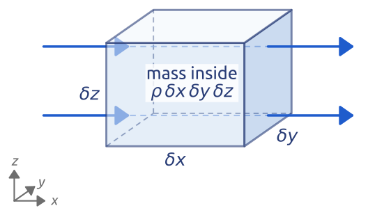
Bookkeeping: what is inside changes only by what crosses the walls

(Vallis 2017, sec. 1.2.1; Cushman-Roisin and Beckers 2011, sec. 3.1)

Control volume first (Pedro’s choice for the engineers); the parcel view comes after. The same bookkeeping is the finite-volume method (lecture 6).

Mass (2/4): fluxes through two faces

Mass per second through a face: density × normal velocity × area. Per unit area: the mass flux \(\rho u\) (\(\mathrm{kg\,m^{-2}\,s^{-1}}\)); \((\rho u)\big|_x\) is its value on the face at \(x\).

\[\begin{aligned} \text{in at } x&: \quad (\rho u)\big|_x\,\delta y\,\delta z\\ \text{out at } x + \delta x&: \quad (\rho u)\big|_{x+\delta x}\,\delta y\,\delta z\\ &\phantom{:}\quad \approx \Big[(\rho u)\big|_x + {\color{#1f5ccc}{\frac{\partial(\rho u)}{\partial x}\,\delta x}}\Big]\,\delta y\,\delta z \end{aligned}\]

\(\approx\): Taylor expansion across the box, to first order in \(\delta x\)

Net inflow through the two \(x\) faces, in minus out:

\[-\frac{\partial(\rho u)}{\partial x}\,\delta x\,\delta y\,\delta z\]

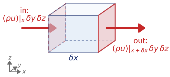
Only the difference between the two faces counts: a divergence of the flux

(Vallis 2017, sec. 1.2.1; Cushman-Roisin and Beckers 2011, sec. 3.1)

(rho u)|_x: the flux at the face at x (a subscript x would be a derivative). Taylor expansion of the flux across the box, first order in dx. Same flux in and out: no change.

Mass (3/4): all six faces

Add the \(y\) and \(z\) faces, divide by \(\delta x\,\delta y\,\delta z\):

\[\frac{\partial\rho}{\partial t} + \frac{\partial(\rho u)}{\partial x} + {\color{#1f5ccc}{\frac{\partial(\rho v)}{\partial y} + \frac{\partial(\rho w)}{\partial z}}} = 0\]

\(\rho\): density; \(\mathbf{u} = (u, v, w)\): velocity

The three flux terms: the divergence of the mass flux, its net outflow per unit volume, \(\nabla\cdot(\rho\mathbf{u}) = \frac{\partial(\rho u)}{\partial x} + \frac{\partial(\rho v)}{\partial y} + \frac{\partial(\rho w)}{\partial z}\).

\[\int_V \nabla\cdot\mathbf{F}\, dV = \oint_{\partial V}\mathbf{F}\cdot\mathbf{n}\, dA\]

\(\mathbf{F}\): any vector field; \(\partial V\): surface of \(V\); \(\mathbf{n}\): outward unit normal

With \(\mathbf{F} = \rho\mathbf{u}\), for any fixed volume:

\[\frac{d}{dt}\int_V \rho\, dV = -\oint_{\partial V}\rho\,\mathbf{u}\cdot\mathbf{n}\, dA\]

The flux form \(\partial_t\rho + \nabla\cdot(\rho\mathbf{u}) = 0\): the starting point of finite volumes

(Vallis 2017, sec. 1.2.1; Cushman-Roisin and Beckers 2011, sec. 3.1)

Integral form: valid for any volume, even with jumps; the differential form needs smooth fields. Finite volumes (lecture 6) discretize exactly this integral balance.

Mass (4/4): following the parcel

With \(\nabla\cdot(\rho\mathbf{u}) = \mathbf{u}\cdot\nabla\rho + \rho\,\nabla\cdot\mathbf{u}\):

\[\begin{gathered}\frac{\partial\rho}{\partial t} + \nabla\cdot(\rho\mathbf{u}) = 0\\ \Big\Updownarrow\\ \frac{D\rho}{Dt} + {\color{#1f5ccc}{\rho\,\nabla\cdot\mathbf{u}}} = 0\end{gathered}\]

• \(\nabla\cdot\mathbf{u}\): how fast a parcel’s volume grows, per unit volume
• Expands (\(\nabla\cdot\mathbf{u} > 0\)): lighter. Compressed: denser
• Water hardly compresses: \(\nabla\cdot\mathbf{u} \approx 0\)
• \(\delta V\) (figure): the volume of a parcel

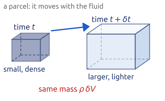
Flux form for a box, advective form for a parcel: the same law

(Vallis 2017, sec. 1.2.2; Cushman-Roisin and Beckers 2011, sec. 3.1)

Product rule. Why does div u measure volume change? Next two slides, following Vallis (2017), 1.1.3 and 1.2.2. Incompressible: the ocean, and the Boussinesq approximation (lecture 3).

A parcel (1/2): its volume

Follow a parcel of volume \(\delta V\). Its surface moves with the fluid: in a time \(\delta t\) a surface element \(dA\) sweeps the volume \((\mathbf{u}\cdot\mathbf{n})\,dA\,\delta t\). Over the whole surface, with the divergence theorem:

\[\frac{D}{Dt}\int_V dV = \oint_{\partial V}\mathbf{u}\cdot\mathbf{n}\,dA = \int_V \nabla\cdot\mathbf{u}\,dV\]

\(V\): a volume moving with the fluid; \(\mathbf{n}\): outward unit normal

For a small parcel:

\[\frac{D\,\delta V}{Dt} = {\color{#1f5ccc}{\nabla\cdot\mathbf{u}}}\;\delta V\]

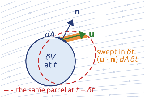
\(\nabla\cdot\mathbf{u}\) is the rate at which a parcel’s volume grows, per unit volume

(Vallis 2017, sec. 1.1.3, eqs. 1.12–1.15)

The surface is material: each element moves with the local u; only the normal part sweeps volume. Small parcel: Vallis (1.15), the limit implied. Incompressible: div u = 0, the volume is kept.

A parcel (2/2): its mass

A parcel keeps its mass, \(\rho\,\delta V\); with \(D\,\delta V/Dt = \delta V\,\nabla\cdot\mathbf{u}\):

\[\begin{aligned}\frac{D(\rho\,\delta V)}{Dt} &= \delta V\,\frac{D\rho}{Dt} + \rho\,\frac{D\,\delta V}{Dt}\\ &= \delta V\,\Big(\frac{D\rho}{Dt} + \rho\,\nabla\cdot\mathbf{u}\Big) = 0\end{aligned}\]

the same equation as for the box. And for any property \(\chi\) per unit mass, as \(\rho\,\delta V\) does not change (transport theorem):

\[\frac{D}{Dt}\int_V \rho\,\chi\, dV = \int_V \rho\,{\color{#1f5ccc}{\frac{D\chi}{Dt}}}\, dV\]

\(\chi\): any property per unit mass: temperature, a velocity component, …; \(V\) moves with the fluid

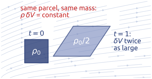
The amount of \(\chi\) in a moving piece of fluid changes only as \(\chi\) changes along each parcel

(Vallis 2017, sec. 1.1.3, eq. 1.21, and sec. 1.2.2, eqs. 1.31–1.33; the name: Chorin and Marsden 1993, sec. 1.1, p. 10)

Vallis (1.31)-(1.33). The transport theorem is (1.21): rho dV is fixed, so D/Dt of the integral acts on chi only. With chi = u it gives Newton’s law for a finite blob of fluid: next.

The continuity equation: two views

Fixed in space (Eulerian)

Mass changes by what flows through the faces

\[\frac{\partial\rho}{\partial t} + \nabla\cdot(\rho\mathbf{u}) = 0\] \[\frac{d}{dt}\int_V \rho\, dV = -\oint_{\partial V}\rho\,\mathbf{u}\cdot\mathbf{n}\, dA\]

\(\partial/\partial t\): at a fixed point; \(V\) fixed in space

Following a parcel (Lagrangian)

Mass kept; volume grows at the rate \(\nabla\cdot\mathbf{u}\)

\[\frac{D\rho}{Dt} + \rho\,\nabla\cdot\mathbf{u} = 0\] \[\frac{D}{Dt}\int_V \rho\, dV = 0\]

\(D/Dt\): following the parcel; \(V\) moves with the fluid

One law of mass conservation: linked by \(D/Dt = \partial_t + \mathbf{u}\cdot\nabla\) and \(\nabla\cdot(\rho\mathbf{u}) = \mathbf{u}\cdot\nabla\rho + \rho\,\nabla\cdot\mathbf{u}\)

(Vallis 2017, sec. 1.2, eqs. 1.27 and 1.33)

The same law seen from two frames. The flux form is what finite volumes discretize (exact conservation on each cell); the advective form is what a parcel feels (Lagrangian and semi-Lagrangian schemes).

Momentum (1/4): Newton for a parcel

Mass × acceleration = forces. With the transport theorem (\(\chi = \mathbf{u}\)):

\[\rho\,\delta V\,\frac{D\mathbf{u}}{Dt} = {\color{#1f5ccc}{\text{body forces} + \text{surface forces}}}\]

• Body forces act on every bit of mass: gravity, \(\rho\,\mathbf{g}\,\delta V\) (\(\mathbf{g}\): gravity per unit mass)
• Surface forces act on the faces: pressure (normal), friction (along the faces)

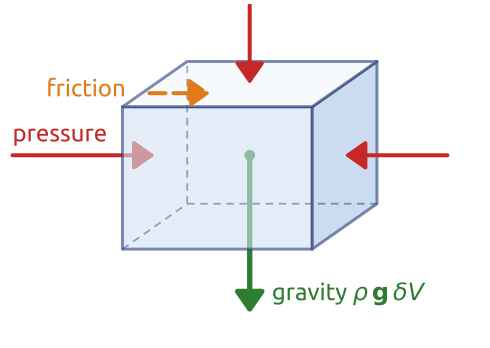
The acceleration is \(D\mathbf{u}/Dt\): following the parcel, not at a fixed point

(Vallis 2017, sec. 1.3; Cushman-Roisin and Beckers 2011, sec. 3.2)

Newton’s second law holds for a parcel, a body made of the same particles. Next: the pressure force on a box, then gravity and friction.

Momentum (2/4): the pressure force

Pressure pushes each face inwards, with force pressure × area. On the two \(x\) faces:

\[\big[p\big|_x - p\big|_{x+\delta x}\big]\,\delta y\,\delta z \approx {\color{#1f5ccc}{-\frac{\partial p}{\partial x}}}\,\delta x\,\delta y\,\delta z\]

All faces, per unit mass (\(\div\,\rho\,\delta V\)):

\[-\frac{1}{\rho}\nabla p\]

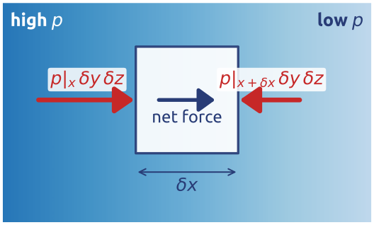
Only pressure differences push: the force points from high to low pressure

(Vallis 2017, sec. 1.3.2; Holton 2004, sec. 1.4)

Ask first: the air around us pushes with 10 tons per square metre. Why are we not crushed, and why does uniform pressure not move the air? (Equal and opposite on opposite faces.) Same Taylor step as for the mass flux.

Momentum (3/4): gravity and friction

Gravity: a body force, \(\mathbf{g} = -g\,\mathbf{k} = -\nabla\Phi\), the gradient of the geopotential \(\Phi = gz\) (\(z\): height; \(\mathbf{k}\): upward unit vector; \(g = 9.81\) m/s²: attraction, plus a small part from the Earth’s turning)

Friction: viscous stresses on the faces. For a fluid like air or water (Navier 1822, Stokes 1845):

\[\mathbf{F} = \nu\,\nabla^2\mathbf{u} \quad (\nabla\cdot\mathbf{u} = 0)\]

\(\nu\): kinematic viscosity: air \(1.5\times10^{-5}\), water \(1.0\times10^{-6}\) m²/s

Reynolds numbers \(Re = UL/\nu \sim 10^{8}\)–\(10^{12}\): molecular friction is negligible at large scales; turbulence is not, and models parameterize it.

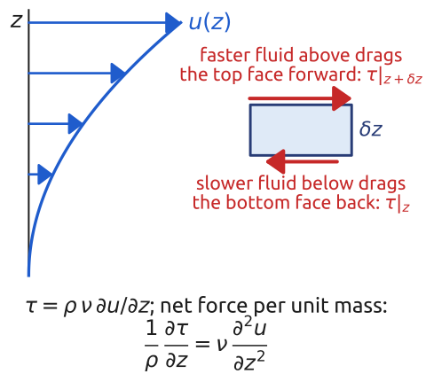
At large scales friction matters mainly near the boundaries: elsewhere, Euler’s equations

(Navier 1827; Stokes 1845; Vallis 2017, sec. 1.3.2; Cushman-Roisin and Beckers 2011, sec. 4.1 and 8.1)

Viscous stress tensor not derived (notes: one paragraph). Re enormous (lecture 1’s scales figure): the flow is turbulent; small eddies carry momentum much better than molecules (eddy viscosity, lecture 9: physics).

Momentum (4/4): Euler and Navier–Stokes

\[\frac{D\mathbf{u}}{Dt} = -\frac{1}{\rho}\nabla p - \nabla\Phi + \mathbf{F}, \qquad \frac{\partial\rho}{\partial t} + \nabla\cdot(\rho\mathbf{u}) = 0\]

• \(\mathbf{F}\): friction. With \(\mathbf{F} = 0\): Euler’s equations (Euler, 1755; printed 1757), derived: Newton’s law for every parcel, the pressure on a box, gravity
• With \(\mathbf{F} = \nu\nabla^2\mathbf{u}\): the Navier–Stokes equations (Navier 1822, Stokes 1845)
• Four equations (three components and mass) for five unknowns \(u, v, w, p, \rho\): thermodynamics is still missing

But: this holds in a frame that does not rotate, and we measure winds on the turning Earth: Coriolis (1835).

Momentum: acceleration of a parcel = pressure force + gravity + friction

(Euler 1757; Chorin and Marsden 1993, sec. 1.1; Vallis 2017, sec. 1.3)

Euler, Berlin 1755: “Principes généraux du mouvement des fluides”, printed 1757 (translation: Frisch, arXiv 0802.2383). His portrait is in lecture 1. Next: Coriolis’s problem, the rotating frame.

Rotating frame (1/4): a vector on the table

A vector \(\mathbf{C}\) fixed on a table turning at \(\boldsymbol{\Omega}\). Seen from space, its tip moves on a circle, at right angles to \(\boldsymbol{\Omega}\) and \(\mathbf{C}\):

\[\left(\frac{d\mathbf{C}}{dt}\right)_{\!I} = {\color{#1f5ccc}{\boldsymbol{\Omega}\times\mathbf{C}}}\]

\((\;)_I\): seen from space (inertial frame)

Size: \(\Omega\,|\mathbf{C}|\sin\theta\), the radius of the circle times the turning rate.

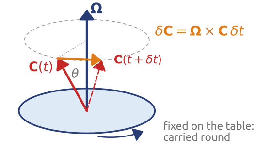
A vector at rest on a turning table changes, seen from space, at the rate \(\boldsymbol{\Omega}\times\mathbf{C}\)

(Vallis 2017, sec. 2.1.1; Cushman-Roisin and Beckers 2011, sec. 2.1)

I: inertial frame (space), R: rotating frame (the table, the Earth). Right-hand rule as on Day 1. The unit vectors of the table are such vectors: d i/dt = Omega x i, etc.

Rotating frame (2/4): any vector, the velocity

A vector that also changes on the table: write it with the table’s unit vectors, which turn:

\[\left(\frac{d\mathbf{B}}{dt}\right)_{\!I} = \left(\frac{d\mathbf{B}}{dt}\right)_{\!R} + {\color{#1f5ccc}{\boldsymbol{\Omega}\times\mathbf{B}}}\]

\((\;)_I\): from space (inertial frame); \((\;)_R\): on the table (rotating frame)

Apply it to the position \(\mathbf{r}\) of a parcel:

\[\mathbf{u}_I = \mathbf{u}_R + {\color{#1f5ccc}{\boldsymbol{\Omega}\times\mathbf{r}}}\]

\(\mathbf{u}_I\): inertial velocity; \(\mathbf{u}_R = (d\mathbf{r}/dt)_R\): relative velocity

Seen from space: its velocity on the table plus the table’s own velocity there.

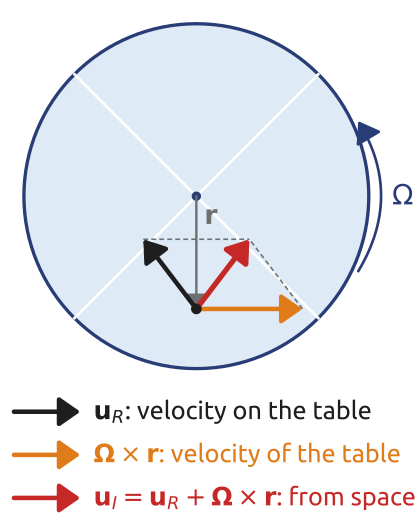
On the Earth, \(\boldsymbol{\Omega}\times\mathbf{r}\) is the ground’s speed: 465 m/s at the equator (Hadley)

(Vallis 2017, secs. 2.1.1–2.1.2, eqs. 2.5 and 2.7; Cushman-Roisin and Beckers 2011, sec. 2.1)

Hadley: lecture 1. B = B1 i + B2 j + B3 k with turning i, j, k: product rule, the derivative of the components is (dB/dt)_R, the derivative of the unit vectors gives Omega x B.

Rotating frame (3/4): the acceleration

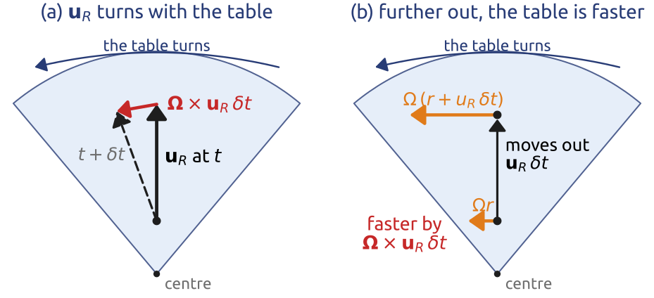
Differentiate \(\mathbf{u}_I = \mathbf{u}_R + \boldsymbol{\Omega}\times\mathbf{r}\) from space, with \((d\mathbf{r}/dt)_I = \mathbf{u}_I\). Apply the rule of the previous slide to \(\mathbf{u}_R\):

\[\begin{aligned} \left(\frac{d\mathbf{u}_I}{dt}\right)_{\!I} &= \left(\frac{d\mathbf{u}_R}{dt}\right)_{\!I} + \boldsymbol{\Omega}\times\mathbf{u}_I\\ &= \left(\frac{d\mathbf{u}_R}{dt}\right)_{\!R} + \underbrace{\boldsymbol{\Omega}\times\mathbf{u}_R}_{\text{(a)}} + \underbrace{\boldsymbol{\Omega}\times\mathbf{u}_R}_{\text{(b)}} + \underbrace{\boldsymbol{\Omega}\times(\boldsymbol{\Omega}\times\mathbf{r})}_{\text{centrifugal}}\\ &= \left(\frac{d\mathbf{u}_R}{dt}\right)_{\!R} + {\color{#1f5ccc}{2\boldsymbol{\Omega}\times\mathbf{u}_R}} + {\color{#1f5ccc}{\boldsymbol{\Omega}\times(\boldsymbol{\Omega}\times\mathbf{r})}} \end{aligned}\]

(a): from the rule applied to \(\mathbf{u}_R\), which turns with the table; (b): from \(\boldsymbol{\Omega}\times\mathbf{r}\) in \(\mathbf{u}_I\), the table’s velocity changes along the parcel’s path (moving outwards, the table is faster there); (a + b): Coriolis acceleration

The factor 2: two equal halves. Hadley kept only (b), the faster ground: half the deflection

(Vallis 2017, sec. 2.1.2, eqs. 2.8–2.12; Persson 1998; Persson 2006)

Vallis 2.8-2.12. (a): u_R turns with the table. (b): Omega x (dr/dt)_I, with (dr/dt)_I = u_R + Omega x r: the parcel reaches points of the table that move differently; plus Omega x (Omega x r), the centripetal acceleration of a point at rest on the table. Hadley (lecture 1) kept the eastward speed in space: only (b) (Persson 1998, 2006).

Rotating frame (4/4): momentum on the Earth

Newton holds in the inertial frame. Move the extra terms to the right-hand side, and drop the subscript \(R\): from now on \(\mathbf{u}\) is the velocity relative to the Earth.

\[\frac{D\mathbf{u}}{Dt} + {\color{#1f5ccc}{2\boldsymbol{\Omega}\times\mathbf{u}}} = -\frac{1}{\rho}\nabla p + \mathbf{g}_{\text{grav}} - {\color{#1f5ccc}{\boldsymbol{\Omega}\times(\boldsymbol{\Omega}\times\mathbf{r})}} + \mathbf{F}\]

\(\mathbf{g}_{\text{grav}}\): Newton’s gravitational attraction, towards the centre of the Earth; \(\mathbf{F}\): friction

• Coriolis force \(-2\boldsymbol{\Omega}\times\mathbf{u}\): turns moving parcels, does no work

• Centrifugal force \(-\boldsymbol{\Omega}\times(\boldsymbol{\Omega}\times\mathbf{r})\): away from the axis, even at rest

But: we never feel the centrifugal force on its own. Why?

Seen from the Earth, two forces appear that come only from our turning point of view

(Vallis 2017, sec. 2.1.3; Persson 1998)

g_grav: Newton’s gravitational attraction (Vallis’s notation, eq. 2.23). Mass and tracer equations do not change in the rotating frame (scalars). Coriolis: Day 1, slides Coriolis and Foucault.

Gravity, centrifugal force, geopotential

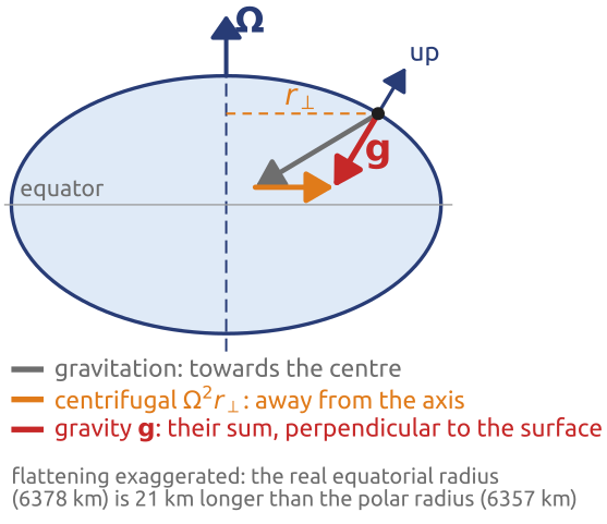
• The centrifugal force is a gradient: \(-\boldsymbol{\Omega}\times(\boldsymbol{\Omega}\times\mathbf{r}) = \Omega^2\mathbf{r}_\perp = -\nabla\Phi_{ce}\), with \(\Phi_{ce} = -\tfrac{1}{2}\Omega^2 r_\perp^2\)
• Added to gravitation, exactly: the effective gravity, gradient of one geopotential \(\Phi\)

\[\mathbf{g} = \mathbf{g}_{\text{grav}} + \Omega^2\mathbf{r}_\perp = -\nabla\Phi\]

\(\mathbf{r}_\perp\): from the axis to the parcel; \(\Phi_{ce}\): centrifugal potential

• Not negligible: only \(\Omega^2 a/g \approx 3\times10^{-3}\) of gravity, but its horizontal part is \(\approx \Omega a/4U \approx 10\) times the Coriolis force (\(a\): Earth’s radius; \(U = 10\) m/s: a typical wind)
• The approximation: “up” along \(\mathbf{g}\), surfaces of constant \(\Phi\) taken as spheres, \(\Phi \approx gz\): a geometric error \(\approx 3\times10^{-3}\)
• It works because the Earth has bulged (21 km) until its surface is nearly a surface of constant \(\Phi\)

\(D\mathbf{u}/Dt + 2\boldsymbol{\Omega}\times\mathbf{u} = -\nabla p/\rho - \nabla\Phi + \mathbf{F}\): the centrifugal force is kept, inside \(\Phi\)

(Vallis 2017, sec. 2.1.2, eq. 2.14, sec. 2.1.3, eq. 2.16, and sec. 2.2.1, eqs. 2.23–2.26; Cushman-Roisin and Beckers 2011, sec. 2.2)

Ask first: the centrifugal force pushes towards the equator. Why does the ocean not pile up there? (The Earth already has: it is oblate.) g = 9.78 at the equator, 9.83 at the poles. Vallis 2.2.1: dropping the horizontal centrifugal force: a large dynamical error (10 x Coriolis); spheres for the geopotential surfaces: a small geometric one.

Notebook Parcels in a rotating frame

Notebook 02b (open in Colab · download): Simulating gravity, centrifugal and Coriolis forces in a rotating frame.

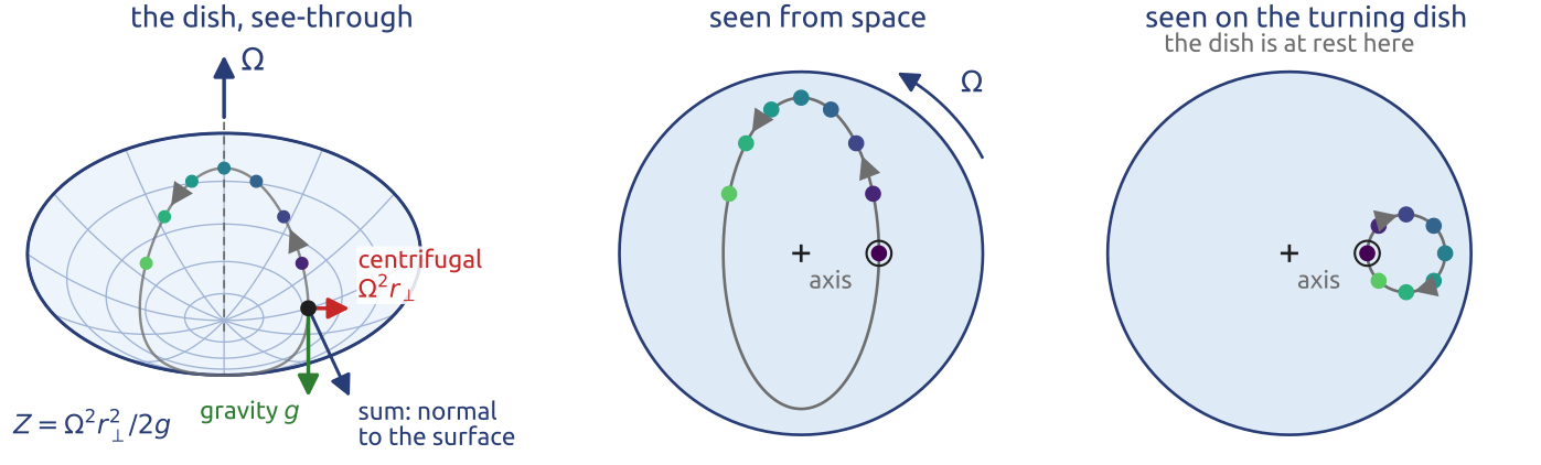
\[-g\nabla Z = -\Omega^2\mathbf{r}_\perp, \qquad Z = \tfrac{1}{2}\Omega^2 r_\perp^2/g\]

\(Z\): height of the dish; \(\mathbf{r}_\perp\): from the axis; \(V\): speed; \(f = 2\Omega\). The slope pulls in as hard as the centrifugal force pushes out

\[\left(\frac{d\mathbf{u}_I}{dt}\right)_{\!I} = -\Omega^2\mathbf{r}_\perp\]

from space: an ellipse, period \(2\pi/\Omega\)

\[\left(\frac{d\mathbf{u}_R}{dt}\right)_{\!R} = -2\boldsymbol{\Omega}\times\mathbf{u}_R\]

on the dish: a circle of radius \(V/f\), period \(2\pi/f\)

One motion: in space the slope pulls the puck back; on the dish the Coriolis force turns it

(Cushman-Roisin and Beckers 2011, secs. 2.2–2.4, eqs. 2.11 and 2.15–2.16; Durran 1993)

Before each run, students write their prediction. The dish is a turning liquid frozen in shape: its surface is a surface of constant geopotential, as the sea (a tank 40 cm across at 30 rpm: 2 cm deeper at the rim, CR&B 2.2). Slope and centrifugal force cancel on the dish, so only Coriolis is left. If time is short: section 2 only.

What the notebook showed

• From space: the slope pulls the puck back to the axis, an ellipse. On the dish, slope and centrifugal force cancel: an inertial circle, once every \(2\pi/f\), \(f = 2\Omega\)
• Under a pressure gradient, from rest: first downhill, then turned to the right (northern hemisphere): inertial oscillations around a drift along the isobars, low pressure on its left: Ferrel’s geostrophic wind \(u_g\) is the average
• Friction damps the oscillations: the drift crosses the isobars towards low pressure

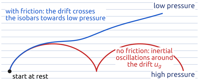
Balance is the average state; the oscillations around it are inertial

(Durran 1993; Cushman-Roisin and Beckers 2011, sec. 2.3)

Real winds near the ground cross the isobars by 10-30 degrees.

Spherical coordinates (1/3): from Cartesian

1. Longitude \(\lambda\), latitude \(\varphi\), radius \(r\); Earth-fixed axes \(X, Y, Z\), \(Z\) along \(\boldsymbol{\Omega}\):

\[\mathbf{r} = r\,(\cos\varphi\cos\lambda,\; \cos\varphi\sin\lambda,\; \sin\varphi)\]

2. Unit vectors (east, north, up) from its derivatives, and the velocity:

\[\mathbf{i} = \frac{1}{r\cos\varphi}\frac{\partial\mathbf{r}}{\partial\lambda},\quad \mathbf{j} = \frac{1}{r}\frac{\partial\mathbf{r}}{\partial\varphi},\quad \mathbf{k} = \frac{\partial\mathbf{r}}{\partial r}\]

\[u = r\cos\varphi\,\frac{D\lambda}{Dt},\quad v = r\,\frac{D\varphi}{Dt},\quad w = \frac{Dr}{Dt}\]

3. The unit vectors turn as the parcel moves:

\[\frac{D\mathbf{u}}{Dt} = \frac{Du}{Dt}\,\mathbf{i} + \frac{Dv}{Dt}\,\mathbf{j} + \frac{Dw}{Dt}\,\mathbf{k} + {\color{#1f5ccc}{u\,\frac{D\mathbf{i}}{Dt} + v\,\frac{D\mathbf{j}}{Dt} + w\,\frac{D\mathbf{k}}{Dt}}}\]

e.g. \(D\mathbf{k}/Dt = (u\,\mathbf{i} + v\,\mathbf{j})/r\); the blue terms give the metric terms

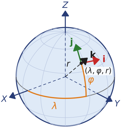
On a sphere the unit vectors depend on the place: following a parcel, they turn

(Vallis 2017, sec. 2.2.2, eqs. 2.36–2.39 (here from the Cartesian components); Holton 2004, sec. 2.3)

Board: i = (-sin lam, cos lam, 0), j = (-sin phi cos lam, -sin phi sin lam, cos phi), k = (cos phi cos lam, cos phi sin lam, sin phi). Gradient: i/(r cos phi) d/dlam + j/r d/dphi + k d/dr. Following the parcel: Di/Dt = u/(r cos phi) (sin phi j - cos phi k), Dj/Dt = -(u tan phi/r) i - (v/r) k, Dk/Dt = (u i + v j)/r.

Spherical coordinates (2/3): grad, div, curl

Edges of the box: \(\delta x = r\cos\varphi\,\delta\lambda\), \(\delta y = r\,\delta\varphi\), \(\delta z = \delta r\)
Areas of its faces: they change with \(\cos\varphi\) and with \(r^2\)

\[\begin{aligned} \nabla &= \frac{\mathbf{i}}{r\cos\varphi}\frac{\partial}{\partial\lambda} + \frac{\mathbf{j}}{r}\frac{\partial}{\partial\varphi} + \mathbf{k}\,\frac{\partial}{\partial r}\\[2pt] \nabla\cdot\mathbf{u} &= \frac{1}{r\cos\varphi}\frac{\partial u}{\partial\lambda} + \frac{1}{r\cos\varphi}\frac{\partial (v\cos\varphi)}{\partial\varphi} + \frac{1}{r^2}\frac{\partial (r^2 w)}{\partial r}\\[2pt] \zeta = \mathbf{k}\cdot\nabla\times\mathbf{u} &= \frac{1}{r\cos\varphi}\Big[\frac{\partial v}{\partial\lambda} - \frac{\partial (u\cos\varphi)}{\partial\varphi}\Big]\\[2pt] \nabla^2 &= \frac{1}{r^2\cos^2\varphi}\frac{\partial^2}{\partial\lambda^2} + \frac{1}{r^2\cos\varphi}\frac{\partial}{\partial\varphi}\Big(\cos\varphi\,\frac{\partial}{\partial\varphi}\Big) + \frac{1}{r^2}\frac{\partial}{\partial r}\Big(r^2\frac{\partial}{\partial r}\Big) \end{aligned}\]

\(\nabla\): divide by the edge lengths; \(\nabla\cdot\): net flux through the faces over the volume \(r^2\cos\varphi\,\delta\lambda\,\delta\varphi\,\delta r\); \(\zeta\): vorticity, the vertical component of the curl: the circulation round the top face over its area; \(\nabla^2 = \nabla\cdot\nabla\)

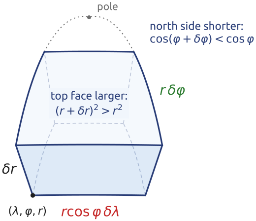
Derivatives along distances, fluxes through faces that shrink to the pole and grow with height

(Vallis 2017, sec. 2.2.2, eqs. 2.27–2.35)

Board: the box of the mass slides, on the sphere. Gradient: divide by the edge lengths. Divergence: flux through east/west faces (area r dphi dr), north/south (r cos phi dlam dr: cos phi inside the derivative), top/bottom (r^2 cos phi dlam dphi: r^2 inside), divided by the volume r^2 cos phi dlam dphi dr. Full curl in the notes (Vallis 2.33); vector Laplacian only via grad div - curl curl (2.34).

Spherical coordinates (3/3): momentum

\[\begin{aligned} \frac{Du}{Dt} - \Big(2\Omega + \frac{u}{r\cos\varphi}\Big)(v\sin\varphi - w\cos\varphi) &= -\frac{1}{\rho\, r\cos\varphi}\frac{\partial p}{\partial\lambda}\\ \frac{Dv}{Dt} + \frac{wv}{r} + \Big(2\Omega + \frac{u}{r\cos\varphi}\Big)u\sin\varphi &= -\frac{1}{\rho\, r}\frac{\partial p}{\partial\varphi}\\ \frac{Dw}{Dt} - \frac{u^2 + v^2}{r} - 2\Omega u\cos\varphi &= -\frac{1}{\rho}\frac{\partial p}{\partial r} - g \end{aligned}\]

\(\dfrac{D}{Dt} = \dfrac{\partial}{\partial t} + \dfrac{u}{r\cos\varphi}\dfrac{\partial}{\partial\lambda} + \dfrac{v}{r}\dfrac{\partial}{\partial\varphi} + w\dfrac{\partial}{\partial r}\); \(u\) east, \(v\) north, \(w\) up

• Metric terms (with \(u/(r\cos\varphi)\), \(wv/r\), \((u^2+v^2)/r\)): the unit vectors \(\mathbf{i}, \mathbf{j}, \mathbf{k}\) turn as the parcel moves
• Thin layers: \(r \to a\) and, together, drop the \(\Omega\cos\varphi\) terms and the metric terms with \(w\)

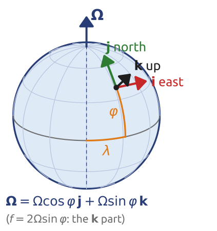
The same law in the coordinates of a sphere: what global models solve

(Vallis 2017, secs. 2.2.3–2.2.4; Holton 2004, sec. 2.3)

Result only; derivation in the notes (unit-vector derivatives). Richardson (1922) wrote these. Thin layers: lecture 3 (scale analysis). Each Coriolis term is a component of 2 Omega x u, with Omega = Omega cos j + Omega sin k.

Thermodynamics (1/5): the gas law

\[p = \rho\,R\,T\]

• Ideal gas, \(T\) in kelvin; \(R = 287\) J/(kg K) for dry air
• Density from pressure and temperature: a fifth equation, but a sixth unknown, \(T\)
• Water vapour changes \(R\) slightly (moist air)

But: what makes \(T\) change? Energy: the first law (Clausius).

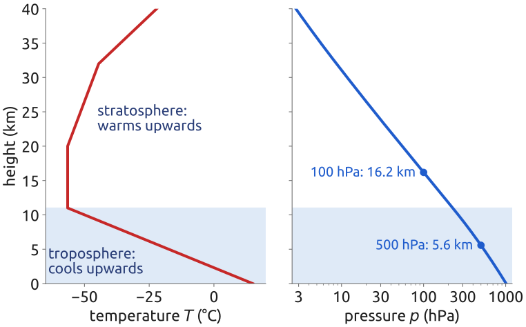
U.S. Standard Atmosphere (1976): pressure halves every 5.5 km or so.

Pressure, density and temperature are tied together: knowing two gives the third

(Vallis 2017, sec. 1.4; NOAA et al. 1976)

R = R*/M = 8.314/0.029 (M: molar mass of dry air, kg/mol). The profiles are computed (formula of the standard atmosphere), not measured on a day. Why pressure falls nearly exponentially: hydrostatic balance (lecture 3).

Thermodynamics (2/5): the first law

Heat added = gain of internal energy + work done in expanding (per unit mass):

\[Q = c_v\frac{DT}{Dt} + {\color{#1f5ccc}{p\,\frac{D\alpha}{Dt}}}\] \(Q\): heating rate (W/kg) by radiation, condensation, conduction; \(c_v = 717\ \mathrm{J/(kg\,K)}\): specific heat at constant volume; \(\alpha = 1/\rho\): specific volume

With \(p\alpha = RT\) and \(c_p = c_v + R\):

\[c_p\frac{DT}{Dt} - \frac{1}{\rho}\frac{Dp}{Dt} = Q\] \(c_p = 1004\ \mathrm{J/(kg\,K)}\): specific heat at constant pressure

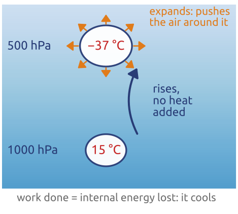
Adiabatic: \(Q = 0\), no heat exchanged. \(T\) still changes: expansion cools, compression warms.

A rising parcel expands and cools even without losing heat: −37 °C at 500 hPa from 15 °C

(Vallis 2017, sec. 1.6.1; Holton 2004, sec. 2.6)

p D(alpha)/Dt = R DT/Dt - alpha Dp/Dt (differentiate p alpha = R T). Board: three lines. Ask: adiabatic means constant T? No: no heat exchanged; T changes by expansion work. Clouds: rising air cools until its water vapour condenses (then Q is no longer 0).

Thermodynamics (3/5): potential temperature

Definition: \(\theta\) is the temperature a parcel would have if moved adiabatically (\(Q = 0\)) to \(p_0 = 1000\) hPa.

On the way, the first law with \(Q = 0\), divided by \(T\), and \(\frac{1}{\rho T} = \frac{R}{p}\) (gas law): \(c_p\,d\ln T = R\,d\ln p\). From \((T, p)\) to \((\theta, p_0)\): \[\int_T^{\theta} c_p\,d\ln T - \int_p^{p_0} R\,d\ln p = 0 \quad\Rightarrow\quad \ln\frac{\theta}{T} = \frac{R}{c_p}\,\ln\frac{p_0}{p}\]

\[\theta = T\left(\frac{p_0}{p}\right)^{R/c_p}\] \(R/c_p = 0.286\) for dry air

• A function of \(T\) and \(p\): every parcel has a \(\theta\)
• \(\theta\) grows upwards: stable

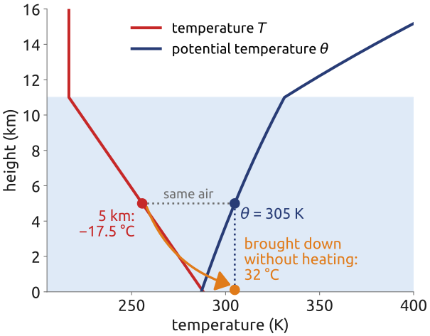
\(\theta\) takes out the cooling by expansion: air at 5 km, at −17.5 °C, has \(\theta = 305\) K

(Vallis 2017, sec. 1.6.1, eqs. 1.103–1.105; Holton 2004, sec. 2.7)

Ask first: air at 5 km is at -17.5 C. Brought down to the ground without heating, how warm is it? (32 C: theta = 305 K, the orange dot of the figure.) Foehn winds. Q = 0 here is an imagined move: it defines theta. Whether the real flow keeps theta: next slide.

Thermodynamics (4/5): how \(\theta\) changes

Now follow the real flow, with any heating \(Q\). Take the logarithm of \(\theta\) and its material derivative:

\[ \begin{aligned} \ln\theta &= \ln T - \frac{R}{c_p}\ln p + \text{const}\\[4pt] c_p\frac{D\ln\theta}{Dt} &= \frac{c_p}{T}\frac{DT}{Dt} - \frac{R}{p}\frac{Dp}{Dt}\\[4pt] &= \frac{1}{T}\left(c_p\frac{DT}{Dt} - \frac{1}{\rho}\frac{Dp}{Dt}\right) && \text{gas law: } \tfrac{R}{p} = \tfrac{1}{\rho T}\\[4pt] &= \frac{Q}{T} && \text{first law} \end{aligned} \]

With \(D\ln\theta/Dt = (1/\theta)\,D\theta/Dt\):

\[\frac{D\theta}{Dt} = \frac{\theta}{c_p T}\,Q\]

• Adiabatic flow, \(Q = 0\): \(\dfrac{D\theta}{Dt} = 0\), \(\theta\) is kept
• Heating raises \(\theta\), cooling lowers it

\(\theta\) labels a parcel: in adiabatic motion it is carried unchanged, like a tracer

(Vallis 2017, sec. 1.6.1, eqs. 1.106–1.108; Holton 2004, sec. 2.7)

Board: the four lines. Q = 0 twice: an imagined move defined theta (previous slide); adiabatic real flow keeps it (this slide). Entropy: d(eta) = c_p d(ln theta), so adiabatic = isentropic. Stability, N: lecture 4.

Thermodynamics (5/5): seawater

• Density depends on temperature, salinity \(S\) (g of salt per kg) and pressure: \(\rho = \rho(T, S, p)\), an empirical formula (TEOS-10)
• Near a reference state, linear:

\[\rho = \rho_0\big[1 - \beta_T(T - T_0) + {\color{#1f5ccc}{\beta_S(S - S_0)}}\big]\]

\(\rho_0, T_0, S_0\): reference state; \(\beta_T\): thermal expansion coefficient; \(\beta_S\): haline contraction coefficient

• Heat and salt are carried by the water, changed by surface sources (heating, evaporation, rain) and mixing: \(D\theta/Dt = \dot\theta\), \(DS/Dt = \dot S\) (\(\theta\): potential temperature; \(\dot\theta\), \(\dot S\): sources, not time derivatives)

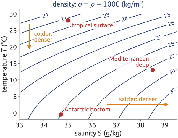
In the ocean salt matters as much as heat: a few kg/m³ drive the deep circulation

(Vallis 2017, sec. 1.4 and 1.7, eqs. 1.96 and 1.141; Cushman-Roisin and Beckers 2011, sec. 3.3)

beta_T ~ 1.7e-4 1/K, beta_S ~ 7.6e-4 per g/kg (Cushman-Roisin & Beckers; Vallis’s notation). Curved contours: the nonlinear real equation (Vallis’s simplified version drawn here). Seawater hardly compresses. In-situ T also changes by compression (about 0.15 K/km): hence theta (Vallis 1.7).

In class: Gibraltar and the deep water

Exercise 2 — Who wins, temperature or salinity? Use the linear equation of state \(\rho = \rho_0\,[1 - \beta_T (T - T_0) + \beta_S (S - S_0)]\) with \(\rho_0 = 1028\) kg/m\(^3\), \(\beta_T = 1.7\times10^{-4}\) K\(^{-1}\), \(\beta_S = 7.6\times10^{-4}\) (g/kg)\(^{-1}\). At Gibraltar, Atlantic water flows into the Mediterranean (15.5 \(^\circ\)C, \(S = 36.2\) g/kg) and Mediterranean water flows out (12.8 \(^\circ\)C, \(S = 38.4\) g/kg). (a) Which water is denser, by how many kg/m\(^3\)? Which one flows out at the bottom? (b) Which difference matters more, temperature or salinity? How warm would the Mediterranean water have to be to flow out on top?

(c) Where does deep water form? Compare warm, salty subtropical surface water (25 \(^\circ\)C, \(S = 37.0\) g/kg) with cold, fresher Labrador Sea water in winter (3 \(^\circ\)C, \(S = 34.9\) g/kg). Which is denser, by how much, and which difference wins here? Where in the ocean would you expect water to sink to the bottom?

In notebook 02c (exercise 1.1): open in Colab · download

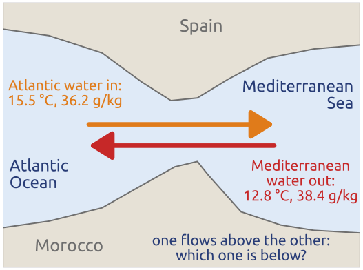
(Cushman-Roisin and Beckers 2011, sec. 3.3 and problem 3.4)

1. d rho/rho0 = -1.7e-4 (12.8 - 15.5) + 7.6e-4 (38.4 - 36.2) = 4.6e-4 + 1.67e-3 = 2.1e-3: Mediterranean denser by 2.2 kg/m3: outflow at the bottom, inflow on top.
2. salinity, 3.6 times; to flow out on top it would have to be above 25.3 C (9.8 K warmer than the Atlantic water, 12.5 K above its own 12.8 C).
3. Labrador denser by 2.2 kg/m3; temperature wins (3.7e-3 vs -1.6e-3): deep water forms in seas where surface water gets cold and salty enough in winter (Greenland, Labrador; Weddell, Ross), not the North Pacific (too fresh). beta_T is smaller in cold water: rough.

The equations of motion, derived

\[\underbrace{\frac{D\mathbf{u}}{Dt}}_{\text{material derivative}} + \underbrace{2\boldsymbol{\Omega}\times\mathbf{u}}_{\text{rotating frame}} = \underbrace{-\frac{1}{\rho}\nabla p}_{\text{pressure on a box}} \underbrace{-\,\nabla\Phi}_{\text{gravity + centrifugal}} + \underbrace{\mathbf{F}}_{\text{friction}}\]

\[\underbrace{\frac{D\rho}{Dt} + \rho\,\nabla\cdot\mathbf{u} = 0}_{\text{mass: box or parcel}} \qquad \underbrace{p = \rho R T, \quad c_p\frac{DT}{Dt} - \frac{1}{\rho}\frac{Dp}{Dt} = Q}_{\text{gas law, first law}} \qquad \underbrace{\frac{Dq}{Dt} = \dot q}_{\text{water vapour}}\]

• Seven equations for the seven unknowns \(u, v, w, p, \rho, T, q\), plus initial and boundary conditions

• Ocean: salinity \(S\) instead of \(q\); \(\rho(T, S, p)\) instead of the gas law; for heat, \(D\theta/Dt = \dot\theta\) instead of the first law

A closed system: seven equations for seven unknowns, for air and for seawater

(Bjerknes 1904; Vallis 2017, Ch. 1–2)

The opening box again, now with today’s derivation under each term. Moisture only mentioned: q is carried by the air, with sources and sinks (evaporation, condensation). F: viscous stress (nu lap u), in practice turbulence, parameterized.

Fast and slow: what the equations allow

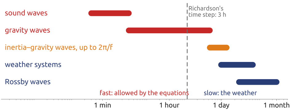
• Sound: compressibility, 340 m/s in air, 1500 m/s in water

• Gravity waves: buoyancy and the free surface, up to 200–300 m/s

• With rotation: inertia–gravity waves, periods up to \(2\pi/f\)

The weather is slow, but the equations also carry fast waves

(Vallis 2017, sec. 1.8 and Ch. 7; Lynch 1999, 2008)

Richardson (lecture 1): his equations (hydrostatic, lecture 3) still had fast gravity waves; his slightly unbalanced start excited them: 145 hPa in 6 h. Had he gone on, his 3 h step (leapfrog over 6 h) would also have been unstable (CFL, lecture 5). Next lecture: filter the fast waves out (scale analysis, hydrostatic balance, shallow water).

Key points

1. \(D/Dt = \partial_t + \mathbf{u}\cdot\nabla\): following a parcel vs. watching a fixed point
2. Mass: \(\partial_t\rho + \nabla\cdot(\rho\mathbf{u}) = 0 \Leftrightarrow D\rho/Dt = -\rho\nabla\cdot\mathbf{u}\); \(\nabla\cdot\mathbf{u}\) is the rate of expansion
3. Momentum on the rotating Earth: \(D\mathbf{u}/Dt + 2\boldsymbol{\Omega}\times\mathbf{u} = -\nabla p/\rho - \nabla\Phi + \mathbf{F}\), with \(\Phi \approx gz\)
4. Heat: \(\theta = T(p_0/p)^{R/c_p}\) is kept in adiabatic motion; seawater: \(\rho(T, S, p)\)
5. Seven equations, seven unknowns; they allow fast waves: sound and gravity waves

Notebooks 02a (open in Colab · download), 02b (open in Colab · download), 02c (open in Colab · download): exercise 1 comes back in 02a, the parcel runs in 02b, exercise 2 in 02c.

Newton’s laws, mass and heat for a fluid on the rotating Earth: a closed system

Reading: (Vallis 2017, secs. 1.1–1.7 and 2.1–2.2; Cushman-Roisin and Beckers 2011, Ch. 2–3)

Next lecture’s warm-up asks about these five. Next: the equations carry sound and gravity waves far faster than the weather. Which terms matter for large, slow motions? Lecture 3.