Reduced models: scales, balance, waves
Atmosphere and Ocean Dynamics, Lecture 3: notes
The equations of motion simplified step by step, keeping the large, slow motions. These notes discuss scale analysis, geostrophic and hydrostatic balance; the scale height, the lapse rate and static stability; the Boussinesq approximation and the primitive equations; the shallow water equations, their potential vorticity, their linear waves (gravity, Poincaré, Kelvin and Rossby waves) and the deformation radius; geostrophic adjustment; quasi-geostrophy and the barotropic vorticity equation; and the Ekman layer, Ekman pumping and the Sverdrup balance of the ocean gyres.
1 Today: keep the slow, large motions
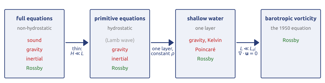
The slide shows a ladder of four models (Figure 1). The full equations of motion, momentum, mass, the gas law and the first law, describe every motion of the air and the sea, including sound waves (minutes), gravity waves (minutes to hours) and inertial oscillations, much faster than the weather (days) or the ocean currents (weeks to years). In Richardson’s forecast of 1922 an initial state slightly out of balance excited these fast waves, and the spurious waves ruined it: 145 hPa in 6 hours (Richardson 1922; Lynch 2008b). The lecture simplifies the equations step by step, each time dropping terms that are small for large, slow motions. A thin fluid (\(H \ll L\), with \(H\) the depth and \(L\) the horizontal size of the motion) is hydrostatic: the primitive equations, without vertically travelling sound waves. One layer of constant density gives the shallow water equations, with gravity, inertia–gravity (Poincaré), Kelvin and Rossby waves. Scales smaller than the deformation radius \(L_d = \sqrt{gH}/f\), the distance a gravity wave travels in a time \(1/f\), make the flow non-divergent: the barotropic vorticity equation of the 1950 forecast, with Rossby waves only. The method, estimating each term and keeping the largest, was made systematic by Charney (1948).
2 Scale analysis (1/4): the equations in components
To compare terms, the momentum equation \(D\mathbf{u}/Dt + 2\boldsymbol{\Omega}\times\mathbf{u} = -\rho^{-1}\nabla p - \nabla\Phi + \mathbf{F}\) is written in components, in local axes at latitude \(\varphi\) on a sphere of radius \(a\): \(x\) eastward, \(y\) northward, \(z\) upward, with velocity components \(u\), \(v\), \(w\) (Holton 2004, sec. 2.3, eqs. 2.19–2.21): \[ \begin{aligned} \frac{Du}{Dt} - 2\Omega v\sin\varphi + 2\Omega w\cos\varphi + \frac{uw}{a} - \frac{uv\tan\varphi}{a} &= -\frac{1}{\rho}\frac{\partial p}{\partial x} + F_x,\\ \frac{Dv}{Dt} + 2\Omega u\sin\varphi + \frac{vw}{a} + \frac{u^2\tan\varphi}{a} &= -\frac{1}{\rho}\frac{\partial p}{\partial y} + F_y,\\ \frac{Dw}{Dt} - 2\Omega u\cos\varphi - \frac{u^2 + v^2}{a} &= -\frac{1}{\rho}\frac{\partial p}{\partial z} - g + F_z . \end{aligned} \tag{1}\] Each equation has an acceleration, Coriolis terms, curvature (metric) terms, the pressure force, gravity in the vertical, and friction, \(\mathbf{F} = \nu\nabla^2\mathbf{u}\) with \(\nu\) the viscosity. Gravity \(g\) includes the centrifugal force, absorbed into the geopotential \(\Phi \approx gz\). The terms in \(1/a\) appear because the local axes turn as a parcel moves over the curved Earth: eastward and northward point in different directions at different places; they come out of the spherical form of the equations (Vallis 2017, sec. 2.2.3).
3 Scale analysis (2/4): the size of each term
Each variable is replaced by a typical size: \(U\) and \(W\) for the horizontal and vertical speeds, \(L\) for the horizontal size of the motion, \(H\) for its depth, \(L/U\) for its time scale (so that \(D/Dt \sim U/L\)), \(\delta P\) for the horizontal pressure changes and \(P_0\) for the surface pressure; \(f_0 = 2\Omega\sin\varphi_0\) at the central latitude \(\varphi_0\); at \(45^\circ\) the factor \(2\Omega\cos\varphi_0\) is as large. Each term of Equation 1 then has a size (Holton 2004, sec. 2.4, Tables 2.1–2.2):
| term (x equation) | \(Du/Dt\) | \(2\Omega v\sin\varphi\) | \(2\Omega w\cos\varphi\) | \(uw/a\) | \(uv\tan\varphi/a\) | \(\rho^{-1}\partial p/\partial x\) | \(F_x\) |
|---|---|---|---|---|---|---|---|
| size | \(U^2/L\) | \(f_0U\) | \(f_0W\) | \(UW/a\) | \(U^2/a\) | \(\delta P/(\rho L)\) | \(\nu U/H^2\) |
| term (z equation) | \(Dw/Dt\) | \(2\Omega u\cos\varphi\) | \((u^2 + v^2)/a\) | \(\rho^{-1}\partial p/\partial z\) | \(g\) | \(F_z\) |
|---|---|---|---|---|---|---|
| size | \(UW/L\) | \(f_0U\) | \(U^2/a\) | \(P_0/(\rho H)\) | \(g\) | \(\nu W/H^2\) |
Two ratios appear. Acceleration over Coriolis is the Rossby number, \((U^2/L)/(f_0U) = U/(f_0L) = Ro\) (Vallis 2017, sec. 2.8.1); depth over size is the aspect ratio \(H/L\), which decides hydrostatic balance (Vallis 2017, sec. 2.7.2).
4 Scale analysis (3/4): the horizontal equations
A mid-latitude weather system at \(45^\circ\)N has \(U = 10\) m/s, \(W = 1\) cm/s, \(L = 1000\) km, \(H = 10\) km (the troposphere), a time scale \(L/U \approx 10^5\) s (about a day), \(\delta P = 10\) hPa, \(\rho \approx 1\) kg/m\(^3\), \(f_0 = 10^{-4}\) s\(^{-1}\), \(a = 6400\) km and the molecular viscosity of air, \(\nu = 1.5\times10^{-5}\) m\(^2\)/s. The terms of the eastward equation are then, in m/s\(^2\), \(10^{-4}\) (acceleration), \(10^{-3}\) (Coriolis with \(v\)), \(10^{-6}\) (Coriolis with \(w\)), \(10^{-8}\) and \(10^{-5}\) (curvature), \(10^{-3}\) (pressure) and \(10^{-12}\) (molecular friction). The slide draws them as bars on a logarithmic scale under each term. The two largest, Coriolis and pressure, balance: the wind is nearly geostrophic, \(f_0 v \approx \rho^{-1}\partial p/\partial x\), \(f_0 u \approx -\rho^{-1}\partial p/\partial y\); the acceleration is \(Ro = 0.1\) of them, so geostrophy holds to about 10 % (Holton 2004, secs. 2.4.1–2.4.2). Being a balance, geostrophy does not say how the flow evolves: for that the small acceleration must be kept. Molecular friction is negligible except very near the ground, where the shear is large.
5 Scale analysis (4/4): the vertical equation
With \(P_0 = 1000\) hPa and \(g \approx 10\) m/s\(^2\), the terms of the vertical equation are \(10^{-7}\) (vertical acceleration), \(10^{-3}\) (Coriolis), \(10^{-5}\) (curvature), \(10\) (pressure force), \(10\) (gravity) and \(10^{-15}\) (friction) (Holton 2004, sec. 2.4.3, Table 2.2). The pressure force balances gravity to better than one part in \(10^4\). This first comparison only shows that the air at rest is hydrostatic. Only pressure differences along the horizontal drive the wind, so what matters is whether the part of the pressure that varies horizontally is hydrostatic too. Split off the state at rest, the horizontal average at each height: \(p = \tilde p(z) + p'\), \(\rho = \tilde\rho(z) + \rho'\), with \(d\tilde p/dz = -\tilde\rho g\) (\(\tilde\rho\) as in Vallis (2017), eq. 2.88c). With \(|\rho'| \ll \tilde\rho\), \[ -\frac{1}{\rho}\frac{\partial p}{\partial z} - g \approx -\frac{1}{\tilde\rho}\left(\frac{\partial p'}{\partial z} + \rho' g\right) \] (Holton 2004, eq. 2.28), and both terms in the bracket are of size \(\delta P/(\tilde\rho H) \sim 10^{-1}\) m/s\(^2\), still a million times the vertical acceleration. The departures of a weather system are hydrostatic too: \[ \frac{\partial p}{\partial z} = -\rho g . \tag{2}\] The vertical velocity can no longer be computed from its own equation; it follows from mass conservation. Hydrostatic balance fails for motions as tall as they are wide (convection, thunderstorms, flow over steep mountains), which kilometre-scale models resolve without this approximation.
Mathematical aside. Hydrostatic balance is the limit of vanishing aspect ratio. Rescaling the vertical coordinate by \(\varepsilon = H/L\), the Navier–Stokes equations in a thin domain (with anisotropic viscosity) converge, as \(\varepsilon \to 0\), to the hydrostatic primitive equations (Azérad and Guillén 2001). The limit is singular: the vertical momentum equation loses its time derivative and \(w\) becomes a diagnostic variable.
6 Hydrostatic balance
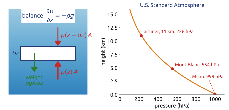
A thin horizontal slab of fluid at rest, of area \(A\) and thickness \(\delta z\) (Figure 2), is pushed up by \(p(z)A\) on its bottom and down by \(p(z + \delta z)A\) on its top, and its weight is \(\rho g A\,\delta z\). Balance gives 1; integrating from \(z\) to the top, \[ p(z) = \int_z^{\infty}\rho g\,dz' : \] the pressure at any level is the weight of the fluid above it, per unit area. At sea level, 1013 hPa is the weight of about 10 tonnes of air per square metre; in the ocean the pressure grows by about 1000 hPa every 10 m of depth. This is why hydrostatic models need no equation to forecast vertical motion, and have no vertically travelling sound waves.
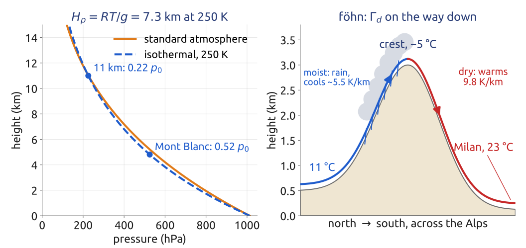
For air, the gas law \(p = \rho RT\), with \(R = 287\) J/(kg K) the gas constant of dry air, gives \[ \frac{1}{p}\frac{\partial p}{\partial z} = -\frac{g}{RT} = -\frac{1}{H_\rho}, \qquad H_\rho = \frac{RT}{g} : \] the pressure falls by a factor \(e\) over the scale height \(H_\rho\), 8.4 km at the 288 K of sea level, 6.5 km at the 223 K of 10 km. In an isothermal atmosphere \(H_\rho\) is constant and \(p = p_0\,e^{-z/H_\rho}\); in general \(p(z) = p_0\exp\big(-\int_0^z g\,dz'/(RT)\big)\). For an isothermal atmosphere \(RT/g\) is both the pressure and the density scale height of Vallis (Vallis 2017, eq. 1.186). Here \(H_\rho = RT/g\) with the local \(T\), strictly the pressure scale height; \(H\) is kept for the depth of a layer.
7 A parcel lifted without heating
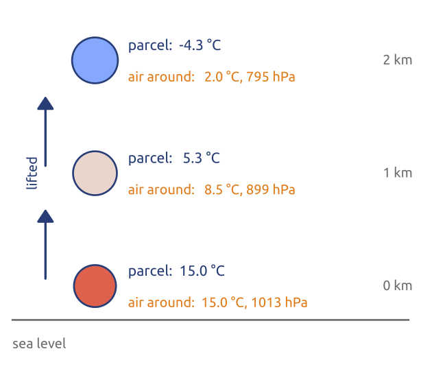
Lift a small parcel of dry air quickly enough that it exchanges no heat with the air around it. At each height its pressure is that of the air around it: the pressure falls, the parcel expands, and expanding, it does work and cools. The first law per unit mass, \(c_p\,DT/Dt - \rho^{-1}Dp/Dt = Q\), with \(c_p = 1004\) J/(kg K) the specific heat of dry air at constant pressure and \(Q\) the heating rate, gives for \(Q = 0\), following the parcel, \(c_p\,dT = dp/\rho\). With the hydrostatic pressure of the air around it, \(dp = -\rho g\,dz\) (the densities of the parcel and of the air nearly equal), \[ \Gamma_d \equiv -\frac{dT}{dz} = \frac{g}{c_p} \approx 9.8\ \text{K/km}, \] the dry adiabatic lapse rate (Holton 2004, sec. 2.7.2, eqs. 2.47–2.48). It is the same for every dry parcel at every height; equivalently, the parcel keeps its potential temperature \(\theta = T(p_0/p)^{R/c_p}\), with \(p_0 = 1000\) hPa. Exactly, keeping \(\theta\), the rate is \((g/c_p)\,T_\text{parcel}/T_\text{air}\), close to \(g/c_p\) since the two temperatures differ by a few per cent.
8 Static stability: vertical displacements of dry air
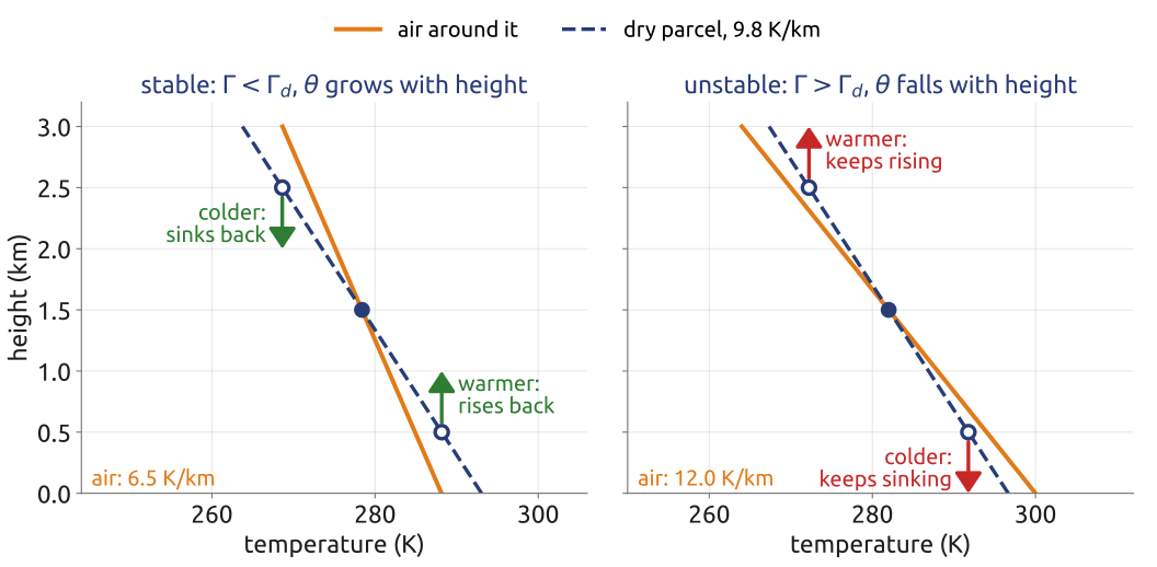
Displace a parcel up or down without heating. If it comes back to its level, the atmosphere is statically stable; if it keeps going, it is unstable, and convection follows. At a given height the parcel has the pressure of the air around it, so by the gas law, \(\rho = p/(RT)\), a parcel colder than its surroundings is denser and sinks, a warmer one is lighter and rises. Lifted, the parcel cools at \(\Gamma_d\); the air around it cools with height at its own lapse rate \(\Gamma = -\partial T/\partial z\). If \(\Gamma < \Gamma_d\), the lifted parcel ends up colder than the air around it and sinks back, and a parcel pushed down ends up warmer and rises back (Figure 4). The logarithm of \(\theta\), with hydrostatic balance and the gas law, gives the criterion (Holton 2004, sec. 2.7.3, eq. 2.49): \[ \frac{T}{\theta}\frac{\partial\theta}{\partial z} = \frac{\partial T}{\partial z} + \frac{g}{c_p} = \Gamma_d - \Gamma , \] so the atmosphere is stable where \(\theta\) grows with height, \(\partial\theta/\partial z > 0\). The parcel keeps its \(\theta\); above its level the air has a higher \(\theta\), so at the same pressure it is warmer than the parcel. The mean atmosphere, cooling by 6.5 K/km, is stable for dry air. Over ground heated by the sun the lowest tens to hundreds of metres can cool faster than \(\Gamma_d\): dry convection, the thermals used by gliders and birds. Moist air is another story: condensation releases heat, a saturated parcel cools more slowly (between about 4 and 6.5 K/km near the ground), and air stable for dry parcels can be unstable for saturated ones (Vallis 2017, sec. 2.10). A stable parcel oscillates about its level; the frequency of this oscillation, the buoyancy frequency, measures the stability.
9 In class: how thick is the atmosphere?
Exercise 1 — How thick is the atmosphere? (a) With hydrostatic balance and the gas law, show that an atmosphere at constant temperature \(T\) has \(p = p_0\,e^{-z/H_\rho}\) with the scale height \(H_\rho = RT/g\). Compute \(H_\rho\) for \(T = 250\) K, and the pressure at Mont Blanc (4808 m) and at 11 km as fractions of \(p_0\). (b) The föhn, a warm, dry wind down the lee side of the Alps (the side sheltered from the wind): dry air crosses them at 3000 m at \(-5\,{}^\circ\)C and comes down to Milan (120 m) without heating. How warm does it arrive? Would an atmosphere cooling by 12 K/km be stable?
Data: \(R = 287\) J/(kg K), \(c_p = 1004\) J/(kg K), \(g = 9.81\) m/s\(^2\); potential temperature \(\theta = T(p_0/p)^{R/c_p}\).
(c) Mars. The Martian atmosphere is carbon dioxide, \(R = 189\) J/(kg K), \(c_p = 770\) J/(kg K), with \(g = 3.71\) m/s\(^2\) and a typical temperature of 210 K. Compute its scale height and its dry adiabatic lapse rate. Its surface pressure is only about 6 hPa: is the Martian atmosphere thinner or thicker than the Earth’s, in kilometres?
10 What the exercise showed
For an isothermal atmosphere at 250 K, \(H_\rho = 287\times250/9.81 = 7.3\) km; the pressure is \(0.52\,p_0\) at Mont Blanc and \(0.22\,p_0\) at 11 km: half the air lies below Mont Blanc, three quarters below cruising airliners (Figure 5, left). The standard atmosphere gives \(0.55\,p_0\) and \(0.22\,p_0\): it is warmer near the ground and colder aloft, and the pressure at a height depends only on the mean of \(1/T\) over the column below it, which up to 11 km is \(1/(251\ \text{K})\). A warm column is thick, a cold one thin; horizontal temperature differences therefore make horizontal pressure differences aloft, which grow with height, and so do the winds they drive, up to the jet stream (the thermal wind). The height of a pressure surface tells the forecaster the mean temperature of the air below it.
The föhn is the warm, dry wind that blows down the lee side of a mountain range (the side sheltered from the wind); the word is the German name, from Latin favonius, used across the Alps, and in the Rocky Mountains the same wind is the chinook. Moist air forced up the windward side cools, its vapour condenses into cloud and rain, and the latent heat makes it cool more slowly than \(\Gamma_d\). Having lost its water, it comes down the other side dry and warms at \(\Gamma_d\): from \(-5\) °C at 3000 m it arrives in Milan (120 m) at about 23 °C, warmer than it was at the same height on the other side (Figure 5, right). An atmosphere cooling by 12 K/km, faster than \(\Gamma_d\), would be unstable. On Mars, with \(R = 189\) J/(kg K), \(c_p = 770\) J/(kg K), \(g = 3.71\) m/s\(^2\) and \(T \approx 210\) K, \(H_\rho = 10.7\) km and \(\Gamma_d = 4.8\) K/km: the Martian atmosphere is thicker than the Earth’s in kilometres, but with a surface pressure of about 6 hPa it holds some 160 kg of air per square metre, against 10 300 kg on the Earth.
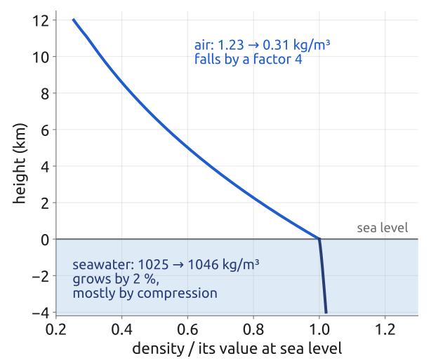
11 The ocean (1/2): density hardly changes
Seawater density varies little. From the surface to the bottom of a 4-km ocean it grows by about 2 %, from about 1025 to 1046 kg/m\(^3\), mostly by compression (Figure 6). Warming by 20 K lowers it by about 0.3 % (thermal expansion coefficient \(\beta_T \approx 1.7\times10^{-4}\) K\(^{-1}\)); adding 5 g/kg of salt raises it by about 0.4 % (haline contraction coefficient \(\beta_S \approx 7.6\times10^{-4}\) (g/kg)\(^{-1}\); typical values for seawater, in the notation of Vallis (2017, eq. 1.57)). Write the density as a constant reference value \(\rho_0\) (about 1027 kg/m\(^3\)) plus a small departure, and the pressure as the hydrostatic pressure of \(\rho_0\) plus a departure (Vallis 2017, eqs. 2.88a, 2.90–2.91): \[ \rho = \rho_0 + \delta\rho, \quad |\delta\rho| \ll \rho_0; \qquad p = \tilde p(z) + \delta p, \quad \frac{d\tilde p}{dz} = -\rho_0 g . \] This is the split used for the air, with the reference density now the constant \(\rho_0\), so \(d\tilde p/dz = -\rho_0 g\). (Vallis writes \(p_0(z)\) for \(\tilde p(z)\); the tilde avoids a clash with the surface pressure \(p_0\).) Start from the momentum equation multiplied by the density, \[ \rho\Big(\frac{D\mathbf{u}}{Dt} + 2\boldsymbol{\Omega}\times\mathbf{u}\Big) = -\nabla p - \rho g\,\mathbf{k} , \] and substitute: since \(\nabla\tilde p = (d\tilde p/dz)\,\mathbf{k} = -\rho_0 g\,\mathbf{k}\) cancels the weight of \(\rho_0\), it becomes, still without approximation (Vallis 2017, eq. 2.93), \[ (\rho_0 + \delta\rho)\Big(\frac{D\mathbf{u}}{Dt} + 2\boldsymbol{\Omega}\times\mathbf{u}\Big) = -\nabla\delta p - g\,\delta\rho\,\mathbf{k} . \] The weight of \(\rho_0\) is held up by \(\tilde p(z)\); only the density anomaly is left to push the water.
12 The ocean (2/2): the Boussinesq equations
Divide by \(\rho_0\). On the left, \(\delta\rho/\rho_0 \sim 10^{-3}\) multiplies the acceleration and can be dropped. On the right, \(g\,\delta\rho/\rho_0\) must be kept: “\(\delta\rho\) may be small, but \(g\) is big” (Vallis 2017, sec. 2.4.2). In mass conservation, \(D\delta\rho/Dt + (\rho_0 + \delta\rho)\nabla\cdot\mathbf{u} = 0\), the first term is \(\delta\rho/\rho_0\) times the size of the second when time scales advectively, so the flow is non-divergent. With a linear equation of state the result is the Boussinesq equations (Vallis 2017, eqs. 2.94, 2.97, 2.101; Cushman-Roisin and Beckers 2011, sec. 3.7): \[ \begin{aligned} \frac{D\mathbf{u}}{Dt} + 2\boldsymbol{\Omega}\times\mathbf{u} &= -\frac{1}{\rho_0}\nabla\delta p + b\,\mathbf{k},\qquad \nabla\cdot\mathbf{u} = 0,\qquad \frac{Db}{Dt} = \dot b,\\ b = -g\,\frac{\delta\rho}{\rho_0} &= g\,\big[\beta_T(T - T_0) - \beta_S(S - S_0)\big], \end{aligned} \] with the buoyancy \(b\), its sources \(\dot b\) (heating, fresh water and salt fluxes), and \(T_0\), \(S_0\) the temperature and salinity of the reference state (Vallis writes \(\phi = \delta p/\rho_0\)). Volume is conserved, so there are no sound waves; \(\nabla\cdot\mathbf{u} = 0\) does not mean that the density of a parcel is constant: it changes by heat and salt, through the equation of state, not by compression.
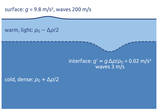
Inside the ocean gravity is felt only through buoyancy. At the thermocline, where warm, light water lies over cold, dense water with a density jump \(\Delta\rho \approx 2\) kg/m\(^3\), a displacement of the interface feels a reduced gravity \(g' = g\,\Delta\rho/\rho_0 \approx 0.02\) m/s\(^2\), five hundred times weaker than \(g\) (Figure 7). Waves on it travel at \(\sqrt{g'H_1} \approx 3\) m/s for an upper layer \(H_1 = 500\) m deep, against 200 m/s for the surface of a 4-km ocean: the internal motions of the ocean are slow, and its eddies small. The atmosphere is not Boussinesq over its whole depth, since its density falls by a factor 3 in 10 km; its models use the anelastic equations or pressure as vertical coordinate, but shallow layers of air are Boussinesq. Boussinesq introduced the approximation in his study of heat convection (1903).
13 Primitive equations (1/2): on the sphere
On the sphere, with longitude \(\lambda\), latitude \(\varphi\) and the distance \(r\) from the centre of the Earth as coordinates, and \(u\), \(v\), \(w\) the eastward, northward and upward velocities, the momentum equation in components is (Vallis 2017, sec. 2.2.3, eqs. 2.45–2.47) \[ \begin{aligned} \frac{Du}{Dt} - 2\Omega v\sin\varphi + 2\Omega w\cos\varphi - \frac{uv\tan\varphi}{r} + \frac{uw}{r} &= -\frac{1}{\rho\,r\cos\varphi}\frac{\partial p}{\partial\lambda},\\ \frac{Dv}{Dt} + 2\Omega u\sin\varphi + \frac{u^2\tan\varphi}{r} + \frac{vw}{r} &= -\frac{1}{\rho\,r}\frac{\partial p}{\partial\varphi},\\ \frac{Dw}{Dt} - 2\Omega u\cos\varphi - \frac{u^2 + v^2}{r} &= -\frac{1}{\rho}\frac{\partial p}{\partial r} - g, \end{aligned} \tag{3}\] with the material derivative \(D/Dt = \partial/\partial t + (u/r\cos\varphi)\,\partial/\partial\lambda + (v/r)\,\partial/\partial\varphi + w\,\partial/\partial r\); \(\rho\) is the density, \(p\) the pressure, \(\Omega\) the rotation rate of the Earth and \(g\) the gravity that includes the centrifugal force. The terms with \(\Omega\) are the Coriolis terms. The quadratic terms in \(1/r\) are the metric terms: the unit vectors that point east, north and up change direction as a parcel moves over the sphere, and the acceleration of the parcel includes the rate of change of the axes (Vallis 2017, eq. 2.44). Moving east along a parallel, for example, the eastward axis turns towards the Earth’s axis, which gives the \(u^2\tan\varphi/r\) term of the northward equation and the \(u^2/r\) part of the vertical one.
For thin, large-scale flow three approximations simplify Equation 3; on the slide they are colour-coded (Vallis 2017, sec. 2.2.4):
- Hydrostatic (green on the slide): the whole left side of the vertical equation is dropped. With the sizes of Section 5, \(Dw/Dt \sim 10^{-7}\) m/s\(^2\), \(2\Omega u\cos\varphi \sim 10^{-3}\) m/s\(^2\) and \((u^2 + v^2)/r \sim 10^{-5}\) m/s\(^2\), against about 10 m/s\(^2\) for the pressure force and for gravity (and \(10^{-1}\) m/s\(^2\) for their departures from the state at rest). The vertical equation becomes
- Shallow fluid (blue): \(r = a + z\), with \(a = 6371\) km the radius of the Earth and \(z\) the height above sea level. The atmosphere that matters for weather lies below 100 km, the ocean is at most 11 km deep: \(r\) is \(a\) to within 2 %. So \(r\) is replaced by \(a\), except where it is differentiated, and \(\partial/\partial r\) becomes \(\partial/\partial z\) (Vallis 2017, eq. 2.49).
- Traditional (red): the Coriolis term \(2\Omega w\cos\varphi\) and the metric terms \(uw/r\) and \(vw/r\) are dropped. They contain \(w \sim 1\) cm/s instead of \(u \sim 10\) m/s: \(2\Omega w\cos\varphi \sim 10^{-6}\) m/s\(^2\), against \(2\Omega v\sin\varphi \sim 10^{-3}\) m/s\(^2\).
14 Primitive equations (2/2): what is left
With the three approximations, Equation 3 becomes (Vallis 2017, sec. 2.2.4, eqs. 2.50–2.51) \[ \begin{aligned} \frac{Du}{Dt} - fv - \frac{uv\tan\varphi}{a} &= -\frac{1}{\rho\,a\cos\varphi}\frac{\partial p}{\partial\lambda},\\ \frac{Dv}{Dt} + fu + \frac{u^2\tan\varphi}{a} &= -\frac{1}{\rho\,a}\frac{\partial p}{\partial\varphi},\\ 0 &= -\frac{1}{\rho}\frac{\partial p}{\partial z} - g, \end{aligned} \tag{4}\] with \(f = 2\Omega\sin\varphi\) the Coriolis parameter and \(D/Dt = \partial/\partial t + (u/a\cos\varphi)\,\partial/\partial\lambda + (v/a)\,\partial/\partial\varphi + w\,\partial/\partial z\). With mass conservation (in the shallow form, with \(a\) for \(r\) (Vallis 2017, eq. 2.52)), the gas law and the first law (Section 7), these are the primitive equations. Only the vertical part of the rotation, \(f\), is left.
The shallow-fluid and the traditional approximations must be made together. With only one of them, the conservation of energy and of angular momentum is not assured; made together, the equations conserve both, with the angular momentum \((\Omega a\cos\varphi + u)\,a\cos\varphi\) (Phillips 1966; Vallis 2017, sec. 2.2.4). Both rest on the small aspect ratio of the motion, so they succeed or fail together. White et al. (2005) derive the whole family of consistent approximations, deep and shallow, hydrostatic and not.
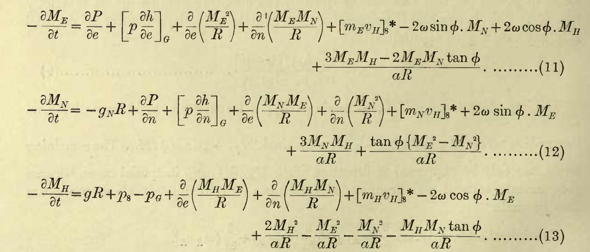
Richardson wrote the same equations in 1922, for the forecast he computed by hand (Figure 8). He kept every term, Coriolis and metric, and put \(a\) for \(a + h\) only (Richardson 1922, Ch. 4/4). His equations are in flux form, for the momentum per unit volume \(\rho u\), and then integrated over a stratum of air; their metric terms differ from those of Equation 4, because on the sphere the divergence in the mass equation adds terms in \(1/a\) of its own. In his words, the terms in \(a^{-1}\) “are derived partly from the centripetal accelerations and partly from the effect of the crowding together of the coordinate lines in the equation of continuity of mass” (p. 32). His \(g_N\) is the north–south component of the apparent gravity at a constant height, directed towards the equator: the centrifugal force of the Earth’s rotation plus the true gravity of an elliptical Earth. He also made his own scale analysis of the vertical equation, writing the size of each term under it: the equation “is nearly equivalent to” hydrostatic balance; the largest of the small terms, the vertical Coriolis term \(2\Omega\rho u\cos\varphi\), “may produce a pressure of 0.5 millibar at sea-level under extreme conditions” (p. 33).
The vertical velocity is diagnosed. With hydrostatic balance, \(w\) has no equation of its own; it follows from mass conservation. In the ocean, Boussinesq, \(\nabla_3\cdot\mathbf{v} = 0\) with \(\mathbf{v} = (u, v, w)\) the 3D velocity and \(\nabla_3\) the 3D gradient, so \(\partial w/\partial z = -\nabla_h\cdot\mathbf{u}_h\), with \(\mathbf{u}_h = (u, v)\) and \(\nabla_h\) the horizontal gradient. Integrated up from a flat bottom at \(z = -H\), where \(w = 0\): \[ w(z) = -\int_{-H}^{z}\nabla_h\cdot\mathbf{u}_h\,dz' . \] In the atmosphere the same is done with pressure as the vertical coordinate. By hydrostatic balance a slab of thickness \(\delta z\) holds the mass \(\rho\,\delta z = -\delta p/g\) per unit area, so a parcel keeps \(\delta x\,\delta y\,\delta p\), and mass conservation takes the form of an incompressible flow (Vallis 2017, sec. 2.6.2, eqs. 2.150–2.152): \[ \nabla_p\cdot\mathbf{u}_h + \frac{\partial\omega}{\partial p} = 0, \qquad \omega = \frac{Dp}{Dt}, \] with \(\nabla_p\) the horizontal gradient at constant pressure and \(\omega\) the vertical velocity in pressure units (Pa/s). With \(\omega = 0\) at the top, \(p = 0\), it gives \(\omega(p) = -\int_0^p\nabla_p\cdot\mathbf{u}_h\,dp'\).
Waves. Sound waves that travel vertically need the vertical acceleration, which hydrostatic balance removes: the primitive equations of the atmosphere have no vertical sound waves. One acoustic mode is left, the Lamb wave, with \(w = 0\): it travels horizontally at about the speed of sound, some 300 m/s; its pressure perturbation and its kinetic energy density decay with height, while its velocity grows (Vallis 2017, sec. 7.8, eqs. 7.214–7.217). In the ocean the primitive equations are made with the Boussinesq equations (\(\rho\) replaced by \(\rho_0\) except in the buoyancy \(b\), \(\nabla_3\cdot\mathbf{v} = 0\)): with no compression at all, there are no sound waves.
Most climate models solve the primitive equations, and almost all ocean models solve their Boussinesq form. So did most global weather prediction models until about a decade ago; since then they have been moving to the non-hydrostatic, compressible equations, needed by grids of a few kilometres, which resolve convection.
15 The f-plane and the beta-plane
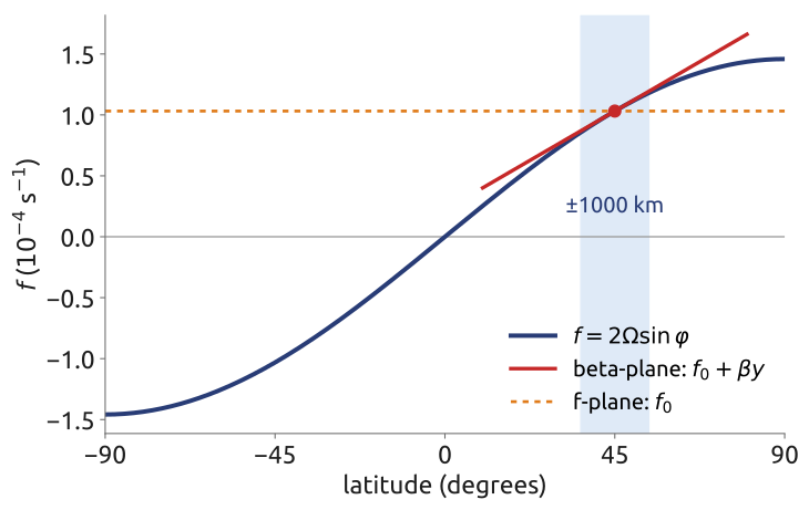
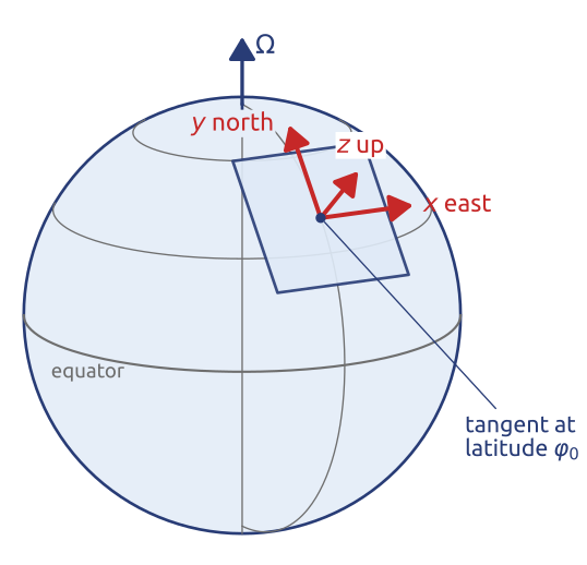
For motions much smaller than the Earth, a flat frame is enough: \(x\) eastward, \(y\) northward, \(z\) upward, on the plane tangent to the Earth at a latitude \(\varphi_0\). The sphere is kept only in the variation of the Coriolis parameter with latitude, expanded to first order in the northward distance \(y = a(\varphi - \varphi_0)\) (Vallis 2017, sec. 2.3.2, eqs. 2.80–2.81): \[ f = 2\Omega\sin\varphi \approx f_0 + \beta y, \qquad f_0 = 2\Omega\sin\varphi_0, \quad \beta = \frac{2\Omega\cos\varphi_0}{a} . \] The f-plane keeps only \(f_0\): at Milan (\(45.5^\circ\)N), \(f_0 = 1.04\times10^{-4}\) s\(^{-1}\). The beta-plane keeps \(\beta y\): at \(45^\circ\), \(\beta = 1.6\times10^{-11}\) m\(^{-1}\)s\(^{-1}\), and over 1000 km \(f\) changes by 15 % (Figure 9). The beta term is small, but it makes the Rossby waves and the narrow western boundary currents of the ocean, such as the Gulf Stream. Rossby introduced the beta-plane in his study of the waves of the mid-latitude flow (Rossby and collaborators 1939). Near the equator, where \(f_0 = 0\), the equatorial beta-plane has \(f = \beta y\).
16 Primitive equations on the beta-plane
On the tangent plane, with \(x = a\lambda\cos\varphi_0\) and \(y = a(\varphi - \varphi_0)\) (Figure 10), the primitive equations Equation 4 become Cartesian (Vallis 2017, sec. 2.3, eqs. 2.78, 2.81–2.83; Cushman-Roisin and Beckers 2011, sec. 9.4): \[ \frac{Du}{Dt} - fv = -\frac{1}{\rho}\frac{\partial p}{\partial x}, \qquad \frac{Dv}{Dt} + fu = -\frac{1}{\rho}\frac{\partial p}{\partial y}, \qquad \frac{\partial p}{\partial z} = -\rho g, \qquad f = f_0 + \beta y , \tag{5}\] with \(D/Dt = \partial/\partial t + u\,\partial/\partial x + v\,\partial/\partial y + w\,\partial/\partial z\). The metric terms \(uv\tan\varphi/a\) and \(u^2\tan\varphi/a\) are dropped: they are of size \(U^2/a\), a fraction \(L/a\) of the acceleration \(U^2/L\), small for motions of size \(L\) well below the radius of the Earth. The Coriolis parameter keeps its variation \(\beta y\) although \(\beta L/f_0\) is small too, because \(\beta\) changes the vorticity dynamics: in Vallis’s words, “sphericity combined with rotation is dynamically equivalent to a differentially rotating system” (Vallis 2017, sec. 2.3.2).
The set is completed differently for the two fluids:
- Atmosphere: mass, \(D\rho/Dt + \rho\,\nabla_3\cdot\mathbf{v} = 0\); the gas law, \(p = \rho RT\); and the first law (Section 7).
- Ocean, Boussinesq (Section 12): \(\rho_0\) for \(\rho\) and the departure \(\delta p\) for \(p\) on the right of the momentum equations; hydrostatic balance of the departures, \(\partial\delta p/\partial z = \rho_0 b\); \(\nabla_3\cdot\mathbf{v} = 0\); and \(Db/Dt = \dot b\).
With \(f = f_0\) these are the f-plane equations, the setting of the shallow water derivation, of the Ekman layer and of quasi-geostrophy below.
17 Shallow water (1/6): one layer
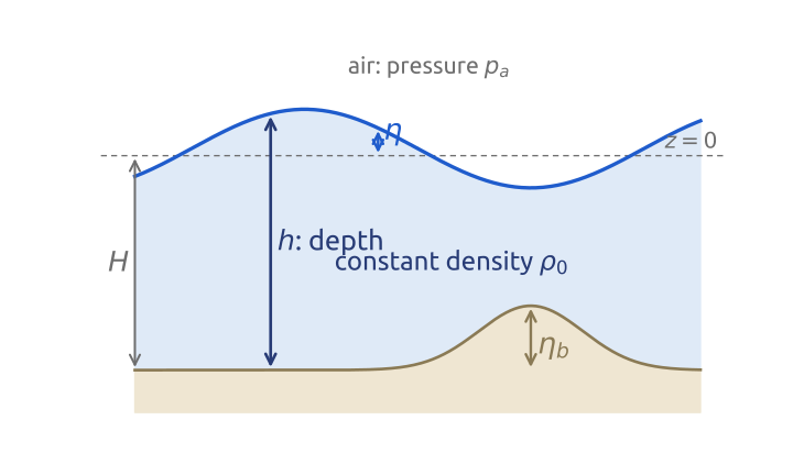
Take a single layer of fluid of constant density \(\rho_0\), thin compared with its horizontal extent (Figure 11). Its free surface is at \(z = \eta(x, y, t)\), above the mean level \(z = 0\); its bottom is at height \(\eta_b(x, y)\) above \(z = -H\), that is at \(z = -H + \eta_b\). Its depth is \[ h = H + \eta - \eta_b . \] Above it, a fluid of negligible density (air over water) exerts a uniform pressure \(p_a\). The unknowns are the horizontal velocity \(\mathbf{u} = (u, v)\) and the depth \(h\) (or \(\eta\)), functions of \(x\), \(y\) and \(t\) only. This is Laplace’s ocean of his tidal theory (1776), the simplest fluid with rotation, gravity waves and balance. It is also a model of the upper ocean above the thermocline (with the reduced gravity \(g'\) for \(g\), Section 12) (Vallis 2017, sec. 3.1; Cushman-Roisin and Beckers 2011, sec. 7.3).
18 Shallow water (2/6): hydrostatic pressure
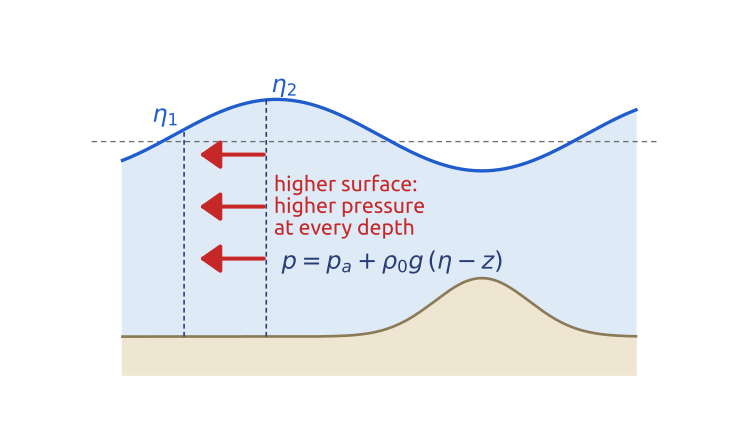
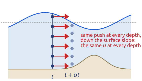
The layer is thin, so it is hydrostatic: \(\partial p/\partial z = -\rho_0 g\). Integrate from a height \(z\) in the fluid up to the surface, where the pressure is that of the air, \(p_a\): \[ \int_z^{\eta}\frac{\partial p}{\partial z'}\,dz' = -\int_z^{\eta}\rho_0 g\,dz' \quad\Longrightarrow\quad p(x, y, z, t) = p_a + \rho_0 g\,\big(\eta(x, y, t) - z\big) \] (Vallis 2017, sec. 3.1.1, eqs. 3.1–3.4, with \(p_a = 0\)). Since \(p_a\) is uniform and \(\rho_0\) constant, the horizontal pressure force per unit mass is \[ -\frac{1}{\rho_0}\nabla p = -g\,\nabla\eta , \] with \(\nabla = (\partial_x, \partial_y)\) the horizontal gradient from here on. It does not depend on \(z\): a higher surface means a higher pressure at every depth below it, by the same amount (Figure 12). If the density varied with depth, the pressure gradient would vary with \(z\) as well.
19 Shallow water (3/6): columns move as columns
Start from the horizontal momentum equation of the primitive equations Equation 5 with constant density, written with the 3D advection, \[ \frac{\partial\mathbf{u}}{\partial t} + (\mathbf{u}\cdot\nabla)\mathbf{u} + w\,\frac{\partial\mathbf{u}}{\partial z} + f\,\mathbf{k}\times\mathbf{u} = -\frac{1}{\rho_0}\nabla p , \] with \(f\,\mathbf{k}\times\mathbf{u} = (-fv, fu)\) and \(\mathbf{k}\) the upward unit vector. The pressure force on the right is \(-g\nabla\eta\), the same at every height. If \(\mathbf{u}\) does not depend on \(z\) at the start, every term of \(\partial\mathbf{u}/\partial t\) is independent of \(z\), and \(\mathbf{u}\) stays independent of \(z\): vertical columns of fluid move as wholes (Figure 13). Then \(w\,\partial\mathbf{u}/\partial z = 0\), although \(w\) itself is not zero (it lifts the surface, Section 20), and \[ \underbrace{\frac{\partial\mathbf{u}}{\partial t}}_{\text{local change}} + \underbrace{(\mathbf{u}\cdot\nabla)\mathbf{u}}_{\text{nonlinear advection}} = \underbrace{-f\,\mathbf{k}\times\mathbf{u}}_{\text{Coriolis}}\;\underbrace{-\,g\nabla(h + \eta_b)}_{\text{pressure}} , \tag{6}\] since \(h + \eta_b = H + \eta\) (Vallis 2017, sec. 3.1.1, eqs. 3.6–3.8; Cushman-Roisin and Beckers 2011, sec. 7.3, eqs. 7.9–7.10). With \(D/Dt = \partial/\partial t + \mathbf{u}\cdot\nabla\), it reads \(D\mathbf{u}/Dt + f\,\mathbf{k}\times\mathbf{u} = -g\nabla\eta\).
This independence of \(z\) comes from hydrostatic balance with constant density, with or without rotation; it is not the Taylor–Proudman effect of rapidly rotating fluids (Vallis 2017, sec. 3.1.1). Friction at the bottom or a wind stress at the top would add terms, and real flows have boundary layers where \(\mathbf{u}\) depends on \(z\).
20 Shallow water (4/6): mass, from the 3D equation
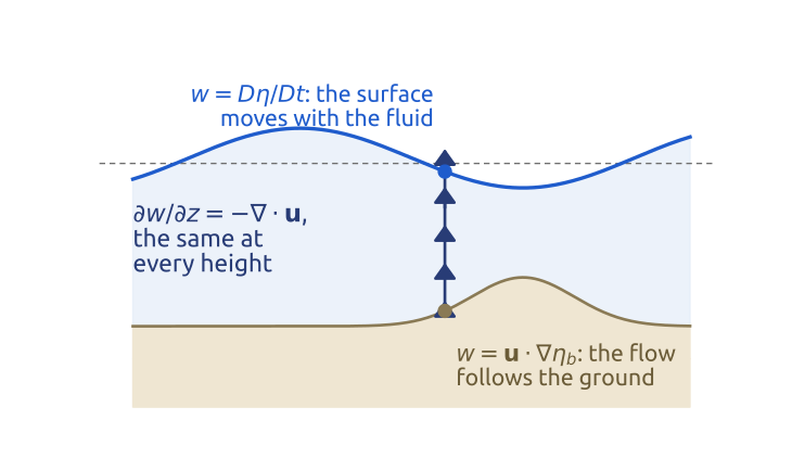
With constant density, mass conservation in 3D is \(\nabla_3\cdot\mathbf{v} = 0\), with \(\mathbf{v} = (u, v, w)\) the 3D velocity and \(\nabla_3\) the 3D gradient: \[ \frac{\partial w}{\partial z} = -\left(\frac{\partial u}{\partial x} + \frac{\partial v}{\partial y}\right) = -\nabla\cdot\mathbf{u} . \] The right side does not depend on \(z\). Integrate from the bottom, \(z_b = -H + \eta_b\), to the surface, \(z = \eta\); the depth is \(\eta - z_b = h\): \[ \int_{z_b}^{\eta}\frac{\partial w}{\partial z}\,dz = -\int_{z_b}^{\eta}\nabla\cdot\mathbf{u}\,dz \quad\Longrightarrow\quad w\big|_{\eta} - w\big|_{z_b} = -h\,\nabla\cdot\mathbf{u} \] (Vallis 2017, sec. 3.1.2, eqs. 3.15–3.16). The kinematic conditions give the vertical velocity at the two boundaries. A particle on the free surface stays on it: its height is \(z_p(t) = \eta(x_p(t), y_p(t), t)\), and by the chain rule its vertical velocity is \[ w\big|_{\eta} = \frac{dz_p}{dt} = \frac{\partial\eta}{\partial t} + u\frac{\partial\eta}{\partial x} + v\frac{\partial\eta}{\partial y} = \frac{D\eta}{Dt} . \] It is \(D/Dt\) and not \(\partial/\partial t\) because the particle also slides along the sloping surface. At the bottom, which does not move, \(\partial\eta_b/\partial t = 0\), yet the flow climbs a bump: \(w|_{z_b} = D\eta_b/Dt = \mathbf{u}\cdot\nabla\eta_b\). Then \[ \frac{D(\eta - \eta_b)}{Dt} = -h\,\nabla\cdot\mathbf{u} , \] and since \(h = H + \eta - \eta_b\) with \(H\) constant, \[ \frac{Dh}{Dt} = -h\,\nabla\cdot\mathbf{u} \quad\Longleftrightarrow\quad \frac{\partial h}{\partial t} + \nabla\cdot(h\mathbf{u}) = 0 , \tag{7}\] by \(\nabla\cdot(h\mathbf{u}) = \mathbf{u}\cdot\nabla h + h\,\nabla\cdot\mathbf{u}\) (Vallis 2017, eqs. 3.17–3.19; Cushman-Roisin and Beckers 2011, sec. 7.3, eqs. 7.11–7.14). Converging columns (\(\nabla\cdot\mathbf{u} < 0\)) get taller: the surface rises.
Inside the column, \(w\) is linear in height, \(w = w|_{z_b} - (\nabla\cdot\mathbf{u})(z - z_b)\) (Vallis 2017, sec. 3.1.4, eq. 3.23) (Figure 14). It follows that the height of a parcel above the bottom, as a fraction of the depth, is kept, \(D[(z - z_b)/h]/Dt = 0\) [eq. 3.27]: a column stretches uniformly.
21 Shallow water (5/6): the equations
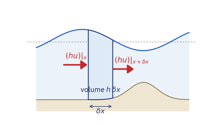
Equation 6 and Equation 7 are the shallow water equations, three equations for \(u\), \(v\) and \(h\) (Vallis 2017, sec. 3.1): \[ \frac{\partial\mathbf{u}}{\partial t} + (\mathbf{u}\cdot\nabla)\mathbf{u} + f\,\mathbf{k}\times\mathbf{u} = -g\nabla(h + \eta_b), \qquad \frac{\partial h}{\partial t} + \underbrace{\mathbf{u}\cdot\nabla h}_{\text{transport}} = \underbrace{-h\,\nabla\cdot\mathbf{u}}_{\text{flow divergence}} . \] The depth at a point changes because columns of another depth are carried there (transport), and because the columns themselves are squeezed or stretched (flow divergence). The flux form \(\partial h/\partial t + \nabla\cdot(h\mathbf{u}) = 0\) is the budget of a fixed column (Figure 15). In one dimension, a column of width \(\delta x\) holds the volume \(h\,\delta x\) per unit width; the volume \((hu)\big|_x\) flows in through its left face per unit time and \((hu)\big|_{x + \delta x}\) out through its right face, so \(\partial(h\,\delta x)/\partial t = (hu)\big|_x - (hu)\big|_{x+\delta x}\), and \(\partial h/\partial t = -\partial(hu)/\partial x\) as \(\delta x \to 0\) (Vallis 2017, eqs. 3.9–3.14). Finite-volume methods start from this form.
Linearized about a fluid at rest over a flat bottom (small \(\eta\) and \(\mathbf{u}\): \((\mathbf{u}\cdot\nabla)\mathbf{u}\) is dropped and \(h\mathbf{u}\) becomes \(H\mathbf{u}\)), they are Laplace’s tidal equations (1776), here without the tidal forcing and on the plane (Hendershott 1981): \[ \frac{\partial\mathbf{u}}{\partial t} + f\,\mathbf{k}\times\mathbf{u} = -g\nabla\eta, \qquad \frac{\partial\eta}{\partial t} + H\,\nabla\cdot\mathbf{u} = 0 . \tag{8}\] They are the standard test problem for the numerical methods of weather and ocean models.
Mathematical aside. Without rotation and in one dimension, \(u_t + uu_x + gh_x = 0\), \(h_t + (hu)_x = 0\) (flat bottom) is a hyperbolic system with characteristic speeds \(u \pm \sqrt{gh}\) (for \(h > 0\)): the same system as the isentropic gas equations with a pressure proportional to the square of the density, \(h\) playing the density (Vallis 2017, sec. 3.1.5). Its discontinuous solutions are hydraulic jumps and bores, the shallow water analogue of shocks. The total energy \(\int\big(\tfrac{1}{2}h|\mathbf{u}|^2 + \tfrac{1}{2}g\eta^2\big)\,dA\) (per unit density, flat bottom) is conserved for smooth solutions, with or without rotation, since the Coriolis force does no work; in the linear case it is \(\tfrac{1}{2}\int(H|\mathbf{u}|^2 + g\eta^2)\,dA\) (Vallis 2017, sec. 3.7.2).
22 Shallow water (6/6): the vector-invariant form
With the relative vorticity \(\zeta = \partial_x v - \partial_y u\) and the kinetic energy per unit mass \(K = |\mathbf{u}|^2/2\), the advection can be rewritten with the vector identity \[ (\mathbf{u}\cdot\nabla)\mathbf{u} = \zeta\,\mathbf{k}\times\mathbf{u} + \nabla K . \] In components: the \(x\) component of the right side is \(-\zeta v + u\,\partial_x u + v\,\partial_x v = -v\,\partial_x v + v\,\partial_y u + u\,\partial_x u + v\,\partial_x v = u\,\partial_x u + v\,\partial_y u\), the \(x\) component of the left; the \(y\) component is checked in the same way. In Equation 6, \(\zeta\) joins \(f\) in front of \(\mathbf{k}\times\mathbf{u}\), and the two gradients join in the Bernoulli potential \(B\): \[ \frac{\partial\mathbf{u}}{\partial t} + (\zeta + f)\,\mathbf{k}\times\mathbf{u} = -\nabla B, \qquad B = \tfrac{1}{2}|\mathbf{u}|^2 + g\,(h + \eta_b) , \] the kinetic plus the potential energy per unit mass. Vallis writes \(B = g\eta + |\mathbf{u}|^2/2\) (Vallis 2017, sec. 3.7.1, eq. 3.94), with his \(\eta\) the height of the surface above the mean bottom, equal to \(h + \eta_b\) here: the same \(B\). Finally, with the potential vorticity \[ Q = \frac{\zeta + f}{h} , \] the spin of a column per unit depth, \((\zeta + f)\,\mathbf{u} = Q\,h\mathbf{u}\), and the shallow water equations read \[ \frac{\partial\mathbf{u}}{\partial t} + Q\,\mathbf{k}\times(h\mathbf{u}) = -\nabla B, \qquad \frac{\partial h}{\partial t} + \nabla\cdot(h\mathbf{u}) = 0 . \tag{9}\] This is the vector-invariant form: it is written with gradient, divergence and curl only, without the advective derivative of the coordinate axes, so it has the same form on the plane and on the sphere (Vallis 2017, sec. 2.2.6, eq. 2.60). Vorticity and potential vorticity are already inside the momentum equation. The same mass flux \(h\mathbf{u}\) appears in both equations; models on C grids, such as MPAS and ICON, discretize this form, and the TRiSK scheme computes \(Q\,\mathbf{k}\times(h\mathbf{u})\) from the same discrete mass flux, so that energy and potential vorticity are conserved on any grid (Ringler et al. 2010; Skamarock et al. 2012).
23 Geostrophic balance in shallow water
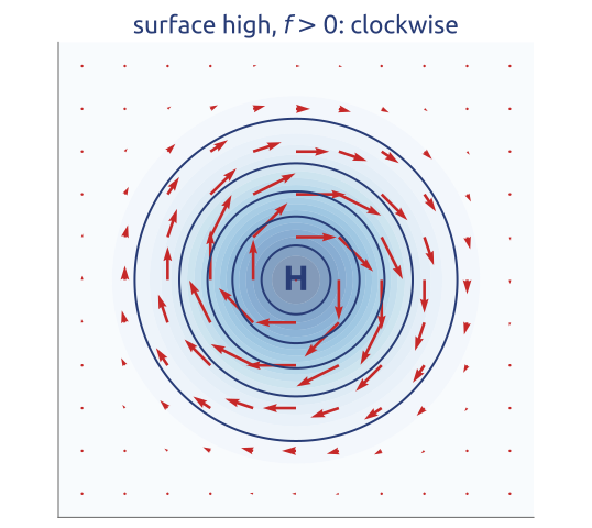
Scale the terms of the momentum equation with a speed \(U\), a size \(L\), the time \(L/U\) and a change \(\delta\eta\) of the surface height over \(L\): \[ \begin{array}{ccccc} \dfrac{\partial\mathbf{u}}{\partial t} + (\mathbf{u}\cdot\nabla)\mathbf{u} & + & f\,\mathbf{k}\times\mathbf{u} & = & -g\nabla\eta\\[6pt] U^2/L & & fU & & g\,\delta\eta/L\\[4pt] Ro & & 1 & & g\,\delta\eta/(fUL) \end{array} \] The last row divides by \(fU\); \(Ro = U/(fL)\) is the Rossby number. For \(Ro \ll 1\) the acceleration is small. The pressure force is then the only term left to balance the Coriolis force, so it must be of order one too: \(\delta\eta \sim fUL/g\). This is not assumed; it follows. With a flatter surface nothing would balance the Coriolis force, which alone would turn the flow round in inertial oscillations; with a steeper one the acceleration would be large, and gravity waves would follow. The balance is geostrophic, with the geostrophic velocity \(\mathbf{u}_g\) (Vallis 2017, secs. 2.8.1–2.8.2, §3.5; Cushman-Roisin and Beckers 2011, sec. 4.5, §7.1): \[ f\,\mathbf{k}\times\mathbf{u}_g = -g\nabla\eta \quad\Longleftrightarrow\quad \mathbf{u}_g = \frac{g}{f}\,\mathbf{k}\times\nabla\eta . \] The flow follows the contours of the surface height, clockwise around a high in the northern hemisphere, fastest where the contours are closest (Figure 16): Ferrel’s geostrophic wind, with the slope of the surface in place of the isobars. For the Gulf Stream, \(U = 1\) m/s and \(L = 100\) km give \(Ro = 0.1\) and \(\delta\eta \approx 1\) m: the surface drops by about a metre across the current, which satellite altimeters measure.
On the f-plane the geostrophic flow has no divergence, \(\nabla\cdot\mathbf{u}_g = 0\), and it flows along the contours of \(\eta\), so by Equation 7 (flat bottom) \(\partial\eta/\partial t = 0\): the surface never changes. Geostrophic balance is a diagnostic relation: it gives the flow from the surface, but not how either evolves. The evolution lies in the small departures from balance, of relative size \(Ro\). To predict, one needs an equation from which the large, balanced terms have been removed: the vorticity equation.
24 Vorticity (1/3): stretching spins up
Start from the vector-invariant momentum equation, \(\partial\mathbf{u}/\partial t + (\zeta + f)\,\mathbf{k}\times\mathbf{u} = -\nabla B\), and take its curl, the operator \(\mathbf{k}\cdot\nabla\times\), which for a horizontal vector \(\mathbf{A} = (A_x, A_y)\) is \(\partial_x A_y - \partial_y A_x\). Term by term:
- \(\mathbf{k}\cdot\nabla\times\partial\mathbf{u}/\partial t = \partial\zeta/\partial t = \partial(\zeta + f)/\partial t\), since \(f\) does not depend on time;
- for any scalar \(a\), \(a\,\mathbf{k}\times\mathbf{u} = (-av, au)\), so \(\mathbf{k}\cdot\nabla\times(a\,\mathbf{k}\times\mathbf{u}) = \partial_x(au) + \partial_y(av) = \nabla\cdot(a\mathbf{u})\); with \(a = \zeta + f\) this is \(\nabla\cdot[(\zeta + f)\,\mathbf{u}]\);
- \(\mathbf{k}\cdot\nabla\times\nabla B = 0\): the curl of a gradient vanishes, and the pressure (the surface slope) and the kinetic energy drop out.
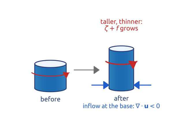
The result is a conservation law for the absolute vorticity \(\zeta + f\), in flux form like Equation 7 for \(h\); expanding the divergence, \(\nabla\cdot[(\zeta + f)\mathbf{u}] = \mathbf{u}\cdot\nabla(\zeta + f) + (\zeta + f)\,\nabla\cdot\mathbf{u}\), gives its advective form (Vallis 2017, sec. 3.7.1, eqs. 3.93–3.95; Cushman-Roisin and Beckers 2011, sec. 7.4): \[ \frac{\partial(\zeta + f)}{\partial t} + \nabla\cdot\big[(\zeta + f)\,\mathbf{u}\big] = 0 \quad\Longleftrightarrow\quad \frac{D(\zeta + f)}{Dt} = -(\zeta + f)\,\nabla\cdot\mathbf{u} . \tag{10}\] The absolute vorticity of a column changes only by convergence or divergence. A column squeezed sideways (converging, \(\nabla\cdot\mathbf{u} < 0\)) gets taller and spins faster, like a skater pulling in her arms (Figure 17). On the beta-plane \(Df/Dt = \beta v\): a column moving north gains planetary vorticity, and to keep \(\zeta + f\) without divergence it must lose relative vorticity.
25 Vorticity (2/3): potential vorticity
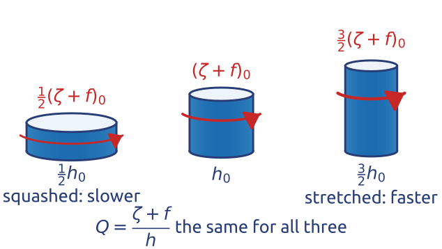
The vorticity equation Equation 10 and mass conservation Equation 7 have the same divergence on the right: \[ \frac{D(\zeta + f)}{Dt} = -(\zeta + f)\,\nabla\cdot\mathbf{u}, \qquad \frac{Dh}{Dt} = -h\,\nabla\cdot\mathbf{u} . \] Eliminate it: for \(Q = (\zeta + f)/h\), by the quotient rule, \[ \frac{DQ}{Dt} = \frac{1}{h}\frac{D(\zeta + f)}{Dt} - \frac{\zeta + f}{h^2}\frac{Dh}{Dt} = -\frac{\zeta + f}{h}\,\nabla\cdot\mathbf{u} + \frac{\zeta + f}{h}\,\nabla\cdot\mathbf{u} = 0 , \] that is (Vallis 2017, sec. 3.7.1, eq. 3.96; Holton 2004, sec. 4.3, eq. 4.13) \[ \frac{D}{Dt}\left(\frac{\zeta + f}{h}\right) = 0 . \tag{11}\] Without forcing and friction, each column keeps its potential vorticity \(Q\): stretched to a larger \(h\) it spins faster, in proportion (Figure 18). It is Kelvin’s circulation theorem for a thin column: its circulation is \((\zeta + f)\) times its cross-section, and its cross-section times \(h\) is its volume, which is kept (Holton 2004, sec. 4.3). Rossby found this conservation for shallow water in 1936 and named the quantity in 1940: “This quantity, which may be called the potential vorticity” (Rossby 1940); Ertel (1942) gave the general form for a stratified fluid (Vallis 2017, sec. 4.5 and the notes to Ch. 4). One scalar field, carried by the flow, holds the slow dynamics: given \(Q\) everywhere and assuming balance, the flow can be recovered.
26 Vorticity (3/3): a column crossing a ridge
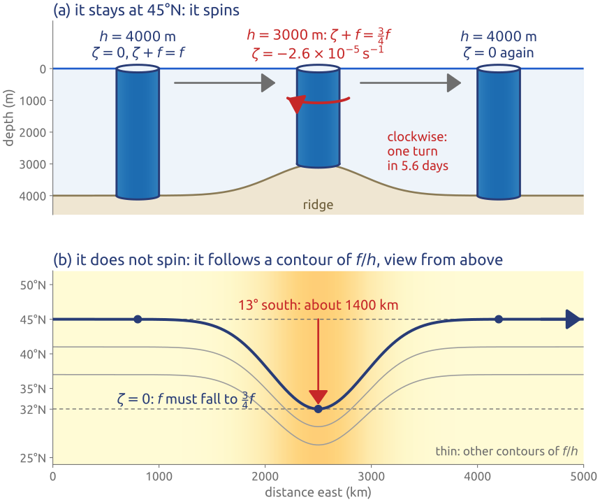
A ridge on the sea floor is an underwater mountain range. Take a column of ocean at \(45^\circ\)N, 4000 m tall and at rest (\(\zeta = 0\)), drifting east over a ridge where the ocean is 3000 m deep (Figure 19). With \(f_0 = f(45^\circ\mathrm{N}) = 2\Omega\sin 45^\circ = 1.03\times10^{-4}\ \mathrm{s^{-1}}\) (\(\Omega = 7.29\times10^{-5}\ \mathrm{s^{-1}}\)), conservation of potential vorticity Equation 11 between the deep floor and the crest gives \[ \frac{\zeta + f}{3000\ \mathrm{m}} = \frac{f_0}{4000\ \mathrm{m}}, \qquad \zeta + f = \tfrac{3}{4}f_0 . \] The column can meet this in two limiting ways (Holton 2004, sec. 4.3).
It stays at \(45^\circ\)N, so \(f = f_0\) and \(\zeta = -\tfrac{1}{4}f_0 = -2.6\times10^{-5}\ \mathrm{s^{-1}}\): it turns clockwise, anticyclonically in the northern hemisphere. For a column turning as a solid body with angular velocity \(\omega\), \(\zeta = 2\omega\), so one turn takes \(4\pi/|\zeta| \approx 4.9\times10^{5}\) s, about 5.6 days.
It does not spin, \(\zeta = 0\), so \(f = \tfrac{3}{4}f_0\): \(\sin\varphi = \tfrac{3}{4}\sin 45^\circ = 0.53\) and \(\varphi = 32^\circ\)N. Over the crest the column has moved \(13^\circ\) of latitude, about 1400 km, towards the equator, and it comes back to \(45^\circ\)N once the ocean is 4000 m deep again. Its path is a contour of \(f/h\), a geostrophic contour: with no relative vorticity, \(f/h\) itself is kept.
In general the column does some of both. Depth and latitude act alike: over large-scale topography the contours of \(f/h\), not the latitude circles, guide the flow, and ocean currents tend to follow the depth contours. The ridge of the example is not extreme: the Mid-Atlantic Ridge rises 2–3 km above an ocean floor 4–5 km deep.
27 Example: eastward winds over the Rockies
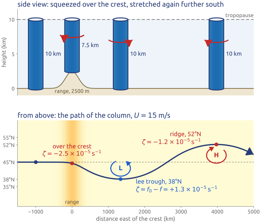
The same argument applies to the air between the ground and the tropopause crossing a mountain range from west to east (Holton 2004, sec. 4.3, Fig. 4.9). Take an eastward wind \(U = 15\) m/s carrying a column at \(45^\circ\)N, 10 km tall, with \(\zeta = 0\), over a north–south range 2500 m high, so that the column is squeezed to 7.5 km over the crest (Figure 20). Its potential vorticity stays \(f_0/10\) km.
Over the crest \(\zeta + f = \tfrac{3}{4}f_0\): the column turns anticyclonically, \(\zeta = \tfrac{3}{4}f_0 - f = -2.5\times10^{-5}\ \mathrm{s^{-1}}\) (the column has already drifted a little south, so \(f\) is slightly below \(f_0\); at \(45^\circ\)N it would be \(-2.6\times10^{-5}\)), and heads towards the equator. Past the range it is 10 km tall again, but further south, where \(f\) is smaller, so \(\zeta = f_0 - f\) is now positive: it turns cyclonically. In the computed path the column reaches \(38^\circ\)N some 1300 km east of the crest, with \(\zeta = f_0 - f(38^\circ\mathrm{N}) = +1.3\times10^{-5}\ \mathrm{s^{-1}}\), then swings north past \(45^\circ\)N to a ridge at \(52^\circ\)N, and so on: a train of troughs and ridges that stands still downstream of the mountains. In the language of weather maps, a trough is a band of low pressure where the flow turns cyclonically (on maps of the height of a pressure surface, the contours dip towards the equator), and a ridge a band of high pressure where it turns anticyclonically (the contours bulge towards the pole). Eastward winds over the Rocky Mountains bend this way, with a ridge of high pressure over the mountains and a trough east of them, the lee trough. A westward wind over the same range gives no such wave downstream (Holton 2004, sec. 4.3, Fig. 4.10).
The path is computed by following the column: it moves at speed \(U\), and its heading turns at the rate \(\zeta/U\) (the relative vorticity of a current turning along a curved path, neglecting the shear across it), with \(\zeta\) from the conservation of \((\zeta + f)/h\) and \(f = 2\Omega\sin\varphi\). The stretching of the column upstream of the range, small for wide ranges (Holton 2004, sec. 4.3), is left out.
28 Linear waves (1/2): an eigenvalue problem
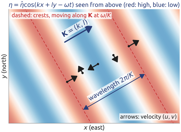
Take Laplace’s equations Equation 8 on the f-plane with a flat bottom, in components: \[ \frac{\partial u}{\partial t} - fv = -g\frac{\partial\eta}{\partial x}, \qquad \frac{\partial v}{\partial t} + fu = -g\frac{\partial\eta}{\partial y}, \qquad \frac{\partial\eta}{\partial t} + H\left(\frac{\partial u}{\partial x} + \frac{\partial v}{\partial y}\right) = 0 . \] Look for plane waves \((u, v, \eta) = (\hat u, \hat v, \hat\eta)\,e^{i(kx + ly - \omega t)}\), with \(\mathbf{K} = (k, l)\) the wavevector, \(\omega\) the frequency and \(\hat u\), \(\hat v\), \(\hat\eta\) the complex amplitudes. Each derivative becomes a factor, \(\partial_t \to -i\omega\), \(\partial_x \to ik\), \(\partial_y \to il\), and the equations become a linear algebraic system (Vallis 2017, sec. 3.8.2, eqs. 3.116–3.118): \[ -i\omega\,\hat u - f\,\hat v + igk\,\hat\eta = 0, \qquad -i\omega\,\hat v + f\,\hat u + igl\,\hat\eta = 0, \qquad -i\omega\,\hat\eta + iHk\,\hat u + iHl\,\hat v = 0 , \] or, in matrix form, \[ \begin{pmatrix} -i\omega & -f & igk\\ f & -i\omega & igl\\ iHk & iHl & -i\omega\end{pmatrix} \begin{pmatrix}\hat u\\ \hat v\\ \hat\eta\end{pmatrix} = \begin{pmatrix}0\\ 0\\ 0\end{pmatrix} . \] The system is homogeneous: if its determinant is not zero, its only solution is the trivial one, \(\hat u = \hat v = \hat\eta = 0\) (no wave). It has a non-zero solution only if the determinant vanishes. Expanding along the first row, \[ \det = i\omega\left(\omega^2 - f^2 - gH(k^2 + l^2)\right) = 0 , \] the dispersion relation [eq. 3.119; Cushman-Roisin and Beckers (2011), §9.1]. For each wavevector \((k, l)\) it has three roots: \(\omega = 0\), the steady geostrophic mode (on the f-plane geostrophic flow has no divergence and satisfies the equations without changing), and two waves travelling in opposite directions. Figure 21 draws one of them.
Mathematical aside. With the energy inner product \(\langle (u, v, \eta), (u', v', \eta')\rangle = \int(Hu\bar u' + Hv\bar v' + g\eta\bar\eta')\,dA\), the linear operator \(\mathcal{L}\) of Equation 8 written as \(\partial_t(u, v, \eta) = \mathcal{L}(u, v, \eta)\) is skew-adjoint: the Coriolis term is skew, and the pressure gradient and the divergence are minus the adjoint of each other after integrating by parts. Its eigenvalues \(-i\omega\) are therefore imaginary: the frequencies are real, the waves neither grow nor decay, and the energy is conserved.
29 Gravity and Poincaré waves
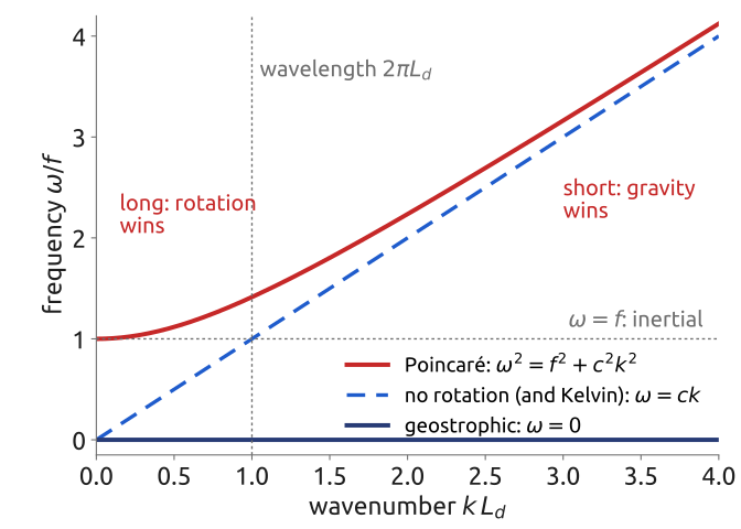
The two roots \(\omega \neq 0\) are the Poincaré waves, or inertia–gravity waves (Vallis 2017, sec. 3.8.2, eqs. 3.120–3.127; Cushman-Roisin and Beckers 2011, sec. 9.3): \[ \omega^2 = \underbrace{f^2}_{\text{inertia}} + \underbrace{c^2(k^2 + l^2)}_{\text{gravity}}, \qquad c = \sqrt{gH} , \] with \(c\) the speed of gravity waves and \(K^2 = k^2 + l^2\). Both restoring effects act: gravity, which flattens the surface, and rotation, which turns the flow. Without rotation, \(f = 0\), they are pure gravity waves, \(\omega = \pm cK\): all wavelengths travel at the same speed \(c\), about 200 m/s in an ocean 4 km deep and 31 m/s in a sea 100 m deep. With rotation, short waves (\(K \gg f/c\)) are still gravity waves, but long waves (\(K \ll f/c\)) become inertial oscillations, \(\omega \to f\), with period \(2\pi/f\) (17 h at \(45^\circ\)N): no wave has a frequency below \(f\). The cross-over is at \(K = f/c\), the wavelength \(2\pi L_d\), with \(L_d = c/f\) (Figure 22). Poincaré waves are dispersive: their group velocity \(d\omega/dK = c^2K/\omega\) is below \(c\) and goes to zero for long waves, which therefore linger near where they were made. The waves are named after Henri Poincaré.
30 Gravity waves seen from space
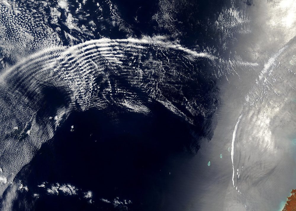
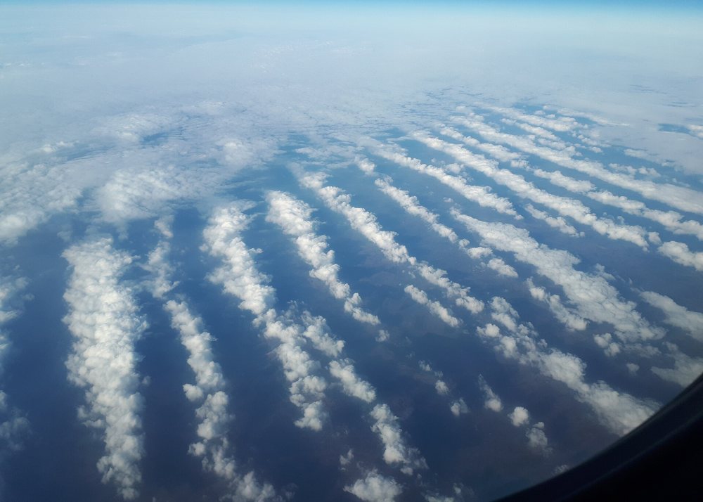
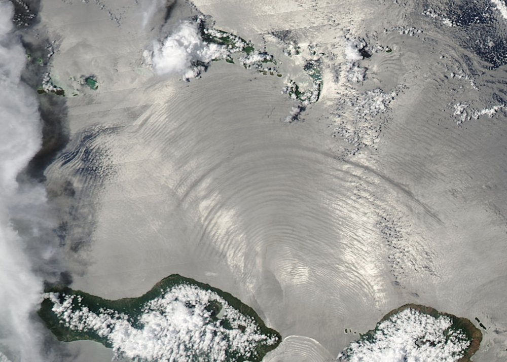
Gravity waves are seen best inside the atmosphere and the ocean, where gravity is reduced. In the atmosphere they show as bands of cloud (Figure 23, Figure 24): air lifted in each crest cools as it expands, its water vapour condenses, and each crest carries a band of cloud; the restoring force is the buoyancy of the stratified air. In the ocean the internal waves travel on the thermocline, the density jump between a warm upper layer and the cold water below (Figure 25). Across a jump \(\Delta\rho\) the interface feels the reduced gravity \(g' = g\,\Delta\rho/\rho_0\): with \(\Delta\rho \approx 2\) kg/m³, \(g' \approx 0.02\) m/s², and over an upper layer of depth \(H = 100\) m, the shallow-water speed is \(c = \sqrt{g'H} \approx 1.4\) m/s, more than a hundred times slower than the surface wave of a 4 km deep ocean, 200 m/s. Rotation does not affect waves of these scales. The waves of Figure 25 are set off by the tidal flow over the rough floor of the Lombok Strait, between Bali and Lombok. Their trace on the surface is faint and shows only in the sunglint, the sunlight reflected back towards the satellite, as bands of rougher and smoother water.



31 The deformation radius
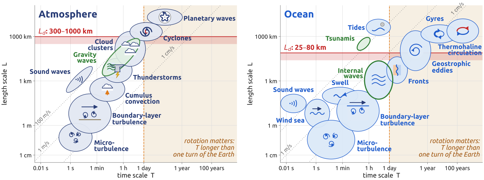
Rotation sets a lowest frequency, \(f\), and a length, \[ L_d = \frac{\sqrt{gH}}{f} , \] the deformation radius (or Rossby radius): the distance a gravity wave travels in a time \(1/f\) (Vallis 2017, sec. 3.9.2; Cushman-Roisin and Beckers 2011, sec. 9.3). For one layer of the full depth it is large: at \(45^\circ\)N (\(f = 1.03\times10^{-4}\) s\(^{-1}\)), about 3000 km for the atmosphere (\(H = 10\) km) and 1900 km for the ocean (\(H = 4\) km). But the atmosphere and the ocean are stratified, and their internal gravity waves are much slower. With the buoyancy frequency \(N\), the frequency at which a displaced parcel oscillates in a stably stratified fluid, and the depth \(H\), the internal gravity-wave speed is \(NH\) and \[ L_d = \frac{NH}{f} , \] about 1000 km in the atmosphere (\(N = 10^{-2}\) s\(^{-1}\), \(H = 10\) km) and 80 km in the ocean (\(N = 2\times10^{-3}\) s\(^{-1}\), \(H = 4\) km) (Vallis 2017, sec. 5.4). The first baroclinic mode of a fluid of constant \(N\), the gravest internal wave, travels at \(c_1 = NH/\pi\); its radius \(L_1 = c_1/f\) is \(\pi\) times smaller, about 300 km and 25 km (Vallis 2017, sec. 12.4, eq. 12.81). Computed from the observed stratification of the ocean, the first radius is some tens of kilometres at mid-latitudes, less at high latitudes and more near the equator (Vallis 2017, fig. 12.13). The reduced-gravity layer of Section 12 gives the same order: \(\sqrt{g'H_1} \approx 3\) m/s and \(L_d \approx 30\) km.
Motions both wider than \(L_d\) and slower than a day are in geostrophic balance: cyclones and planetary waves in the air, eddies and gyres in the sea (Figure 26). The internal radius sets the size of weather systems and of ocean eddies, and the ocean’s “weather” is about ten times smaller than the atmosphere’s.
32 Kelvin waves (1/3): along a coast
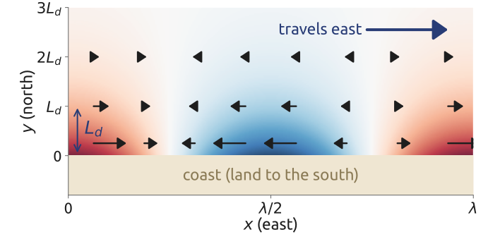
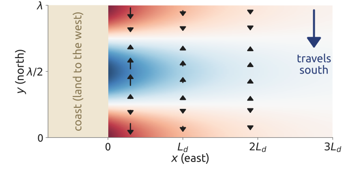
A wall allows one more wave. Take a straight coast along \(y = 0\), with the fluid in \(y > 0\): no flow through the wall. Put \(v = 0\) everywhere in Laplace’s equations (Vallis 2017, sec. 3.8.3, eqs. 3.128–3.135): \[ \frac{\partial u}{\partial t} = -g\frac{\partial\eta}{\partial x}, \qquad f u = -g\frac{\partial\eta}{\partial y}, \qquad \frac{\partial\eta}{\partial t} + H\frac{\partial u}{\partial x} = 0 . \] The first and the third, along the coast, are the equations of a gravity wave in \(x\): try \(\eta = F(x - ct)\,G(y)\), travelling towards \(+x\) with \(c = \sqrt{gH}\) and any shape \(F\); then \(u = (g/c)\,\eta\) satisfies both. The second, across the coast, is a geostrophic balance: with \(u = (g/c)\,F\,G\) it gives \((fg/c)\,G = -g\,G'\), so \[ G' = -\frac{f}{c}\,G, \qquad G = e^{-y/L_d}, \qquad L_d = \frac{c}{f} . \] The wave travelling the other way, \(F(x + ct)\), has \(u = -(g/c)\,\eta\) and needs \(G' = +(f/c)\,G\): it would grow away from the coast, which is impossible. The Kelvin wave is therefore \[ \eta = A\,e^{-y/L_d}\,F(x - ct), \qquad u = \frac{g}{c}\,\eta, \qquad v = 0 , \] with \(A\) the amplitude at the coast (Figure 27). It travels at the gravity-wave speed \(c\), with any shape (no dispersion), trapped within about \(L_d\) of the coast, and one way only: with the coast on its right in the northern hemisphere, on its left in the southern (Thomson 1880; Cushman-Roisin and Beckers 2011, sec. 9.2). Along a coast with the land to the west, the wave keeps the coast on its right by travelling south, \(\eta = A\,e^{-x/L_d}F(y + ct)\), \(v = -(g/c)\,\eta\), \(u = 0\).
33 Kelvin waves (2/3): around a basin, the tides
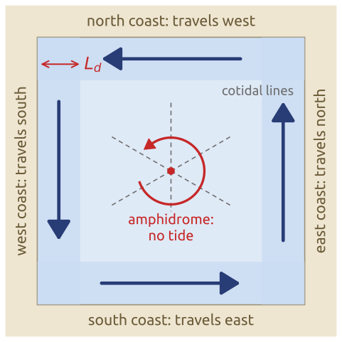
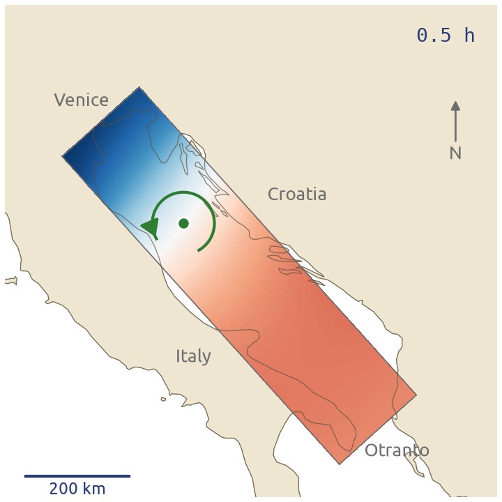
In a closed basin in the northern hemisphere, a Kelvin wave keeps each coast on its right: it travels east along the southern coast, north along the eastern one, west along the northern and south along the western one, so it circles the basin anticlockwise, in the cyclonic sense (Vallis 2017, sec. 3.8.3) (Figure 29). In the southern hemisphere, where \(f < 0\), the coast is on the wave’s left and the waves circle a basin clockwise, again in the cyclonic sense. In a basin a few \(L_d\) wide the waves running along the coasts make the tide turn around an amphidromic point, where the tidal range is zero, with the cotidal lines (lines of equal phase, where high water arrives at the same time) radiating from it (Cushman-Roisin and Beckers 2011, sec. 9.2). For the tide, a barotropic wave, \(L_d = \sqrt{gH}/f\): at \(45^\circ\)N about 200–300 km in a shelf sea 50–100 m deep, and 1900 km in the 4 km deep ocean. In the Adriatic the tide runs up the eastern coast and down the Italian one (Figure 30).
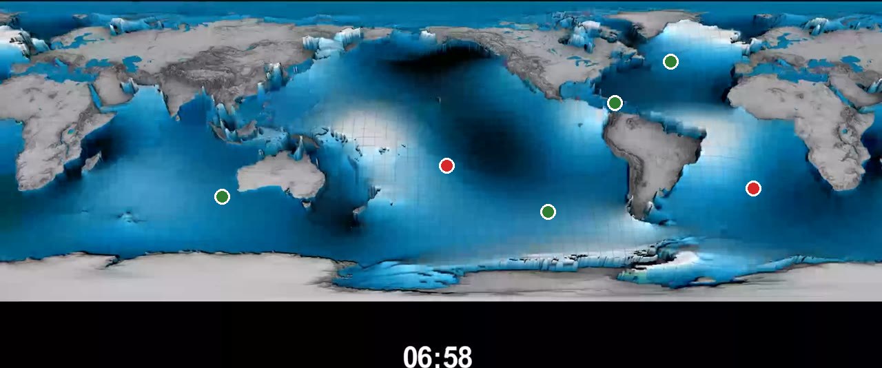
The open oceans are many \(L_d\) wide, and there the picture is less simple: the tides are generated in the deep ocean and spread as Kelvin and inertia–gravity waves (Cushman-Roisin and Beckers 2011, sec. 9.8), which reflect at the coasts and interfere. An amphidromic point is then “a place where the various wave components cancel each other (destructive interference)” (Cushman-Roisin and Beckers 2011, sec. 9.8), and its sense of turning is not set by the hemisphere alone: in the animation of the global tide the amphidromes of the central South Pacific and of the South Atlantic turn anticlockwise, against the sense of the coastal Kelvin wave in the southern hemisphere (Figure 31).
34 Kelvin waves (3/3): the equator as a coast
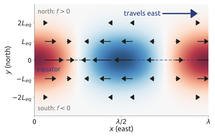
On the equatorial beta-plane, \(f = \beta y\), the Coriolis parameter changes sign at the equator. An eastward wave has the equator on its right in the northern hemisphere, where \(f > 0\), and on its left in the southern, where \(f < 0\): each side is a Kelvin wave of its own hemisphere, and the equator acts as a coast for both. With \(v = 0\) the equations are those of the coastal case with \(f = \beta y\) (Vallis 2017, sec. 8.2, eqs. 8.57a–c); the balance across the equator, \(\beta y\,u = -g\,\partial\eta/\partial y\), gives a Gaussian instead of an exponential: \[ u = G(x - ct)\,e^{-y^2/(2L_{eq}^2)}, \qquad \eta = \frac{H}{c}\,u, \qquad v = 0, \qquad L_{eq} = \left(\frac{c}{\beta}\right)^{1/2} \] (Vallis 2017, eqs. 8.21, 8.62) (Figure 32). The wave travelling west would grow away from the equator: equatorial Kelvin waves travel east only, without dispersion (Matsuno 1966). The equatorial deformation radius \(L_{eq}\) is about 1000 km in the atmosphere (\(c = 25\) m/s, \(\beta = 2.3\times10^{-11}\) m\(^{-1}\) s\(^{-1}\)) and 300 km in the ocean (\(c = 2\) m/s) (Vallis 2017, sec. 8.2, eq. 8.21). Holton writes the decay width as \(Y_K = (2c/\beta)^{1/2}\), 1600 km for \(c = 30\) m/s, the same scale up to a factor \(\sqrt 2\) (Holton 2004, sec. 11.4.2).
In the atmosphere, Kelvin waves are observed in the equatorial stratosphere, mostly of zonal wavenumber 1 with periods of 12–20 days (Holton 2004, sec. 12.5.3), and in the troposphere coupled to convection, as eastward-moving bands of tropical rain whose horizontal structure is Matsuno’s (Kiladis et al. 2009). In the ocean, equatorial Kelvin waves cross the Pacific and are part of El Niño (Vallis 2017, sec. 22.7).
35 Kelvin waves in the air: rain patterns moving east
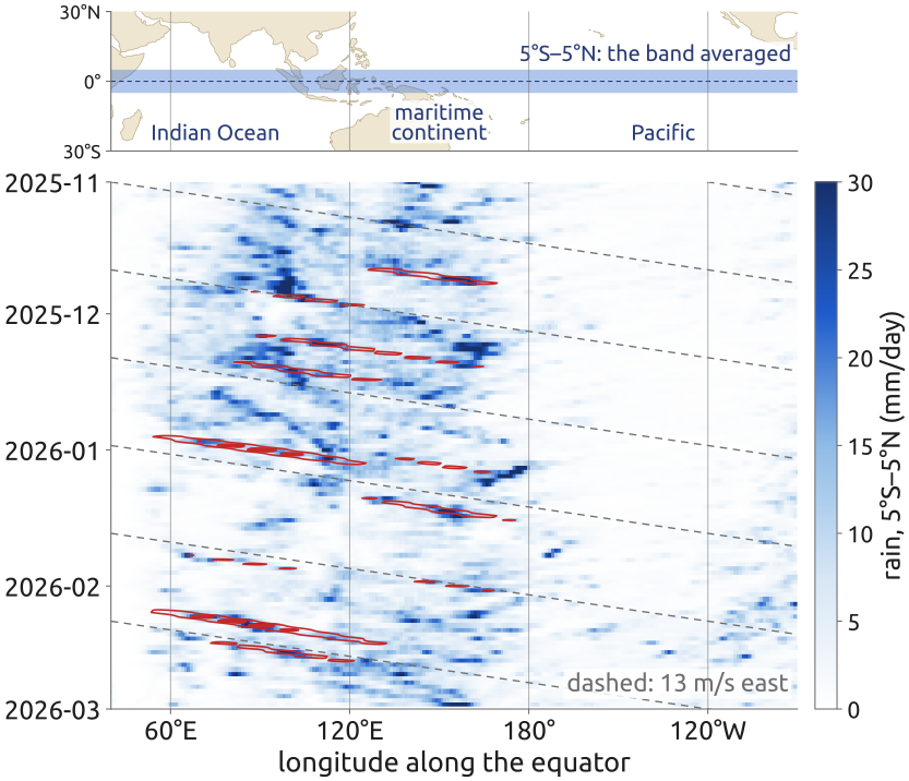
Equatorial Kelvin waves are seen in the weather of the tropics. Figure 33 is a longitude–time (Hovmöller) diagram of the rain along the equator: the ERA5 rain rate (Hersbach et al. 2020), averaged from \(5^\circ\)S to \(5^\circ\)N, day by day from November 2025 to February 2026, with time running down. Many streaks tilt to the right: the pattern of rain moves east, from the Indian Ocean across the maritime continent towards the Pacific. Keeping only the part of the field that moves east with periods of 2.5 to 30 days and zonal wavenumbers 1 to 14 (a two-dimensional Fourier filter in longitude and time), and correlating it with itself one to three days later, gives a speed of about 10° of longitude per day, 13 m/s.
These convectively coupled Kelvin waves have the horizontal structure of Matsuno’s shallow-water solutions, but “their scales do not correspond to that expected from the linear theory of dry waves” (Kiladis et al. 2009): read as a shallow-water Kelvin wave, \(c = \sqrt{gh}\) with \(c = 13\) m/s needs an equivalent depth \(h = c^2/g \approx 17\) m, very much less than the depth of the troposphere. In a stratified fluid each vertical mode has its own equivalent depth, \(c^2/g\); here it is enough that the waves travel east, along the equator, as the theory says.
The trade winds blow towards the west, yet the rain pattern moves east. There is no contradiction: it is not one cloud that travels east with its rain, but the place where clouds form. Each cloud grows, rains and dies where it is, carried by the local wind, while new clouds form further east, where the wave’s convergence lifts the air. Waves don’t carry air, they carry the pattern. In a Kelvin wave the air only sloshes back and forth, eastward under the crests and westward under the troughs, at a few metres per second. And the wave travels at its speed \(c\) relative to the air: in a wind \(U\), it is seen from the ground at \(U + c\), a Doppler shift. Matsuno’s result, eastward only, holds in the frame of the air, whatever the wind; a westward wind only slows the wave as seen from the ground.
36 Rossby waves (1/4): the mechanism
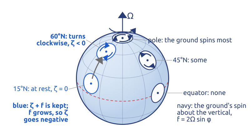
On the rotating sphere a parcel keeps its absolute vorticity \(\zeta + f\) (with no divergence, Equation 10). Carried north, it meets a larger \(f\), so its \(\zeta\) decreases: it turns clockwise relative to the ground (Figure 34). Carried south, it turns anticlockwise.
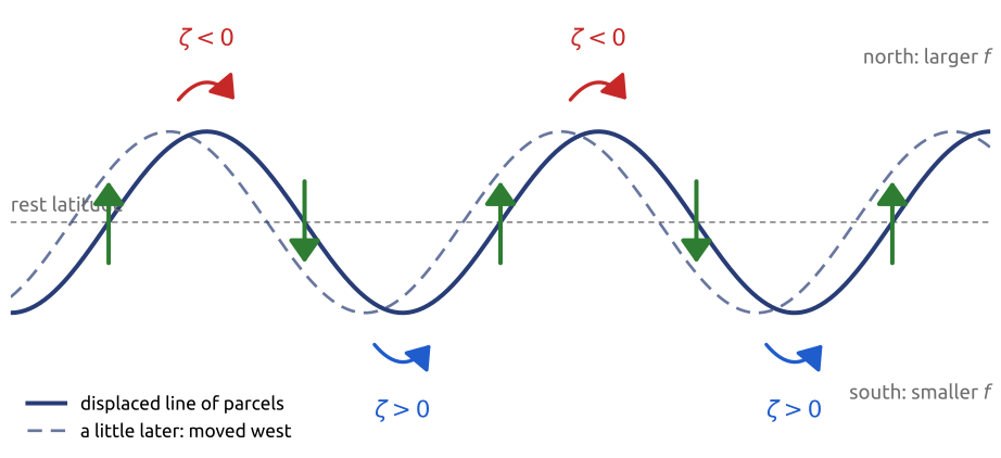
Now displace a line of parcels at rest along a latitude into a wave (Figure 35). Parcels moved north acquire \(\zeta < 0\), parcels moved south \(\zeta > 0\). The spinning parcels push their neighbours: a clockwise vortex at a northward crest drives a northward flow on its west side and a southward flow on its east side; the anticlockwise vortices at the troughs do the same. The line is therefore pushed north just west of each crest and south just east of it: the pattern moves west (Vallis 2017, sec. 6.4.3; Cushman-Roisin and Beckers 2011, sec. 9.4). The restoring effect is the gradient of \(f\), \(\beta\): a gradient of potential vorticity. Any background gradient of potential vorticity does the same, for example a sloping sea floor, which carries topographic Rossby waves.
In equations: take the barotropic vorticity equation, \(D(\zeta + f)/Dt = 0\), on the beta-plane, and linearize it about a uniform eastward wind \(U\). The wave is a small perturbation, with streamfunction \(\psi'\), vorticity \(\zeta' = \nabla^2\psi'\) and northward velocity \(v' = \partial\psi'/\partial x\). The wind carries the perturbation’s vorticity, \(U\,\partial\zeta'/\partial x\), and a parcel moved north by \(v'\) changes its planetary vorticity at the rate \(\beta v'\) (Vallis 2017, sec. 6.4.2, eq. 6.57): \[ \Big(\frac{\partial}{\partial t} + U\frac{\partial}{\partial x}\Big)\zeta' + \beta v' = 0 . \tag{12}\] The term \(\beta v'\) is the mechanism of Figure 35: northward motion makes negative vorticity.
37 Rossby waves (2/4): wind east, waves west
For a plane wave, \(\psi' \propto e^{i(kx + ly - \omega t)}\), Equation 12 gives \(\zeta' = -K^2\psi'\) with \(K^2 = k^2 + l^2\), \(v' = ik\psi'\), and \((-i\omega + iUk)(-K^2) + i\beta k = 0\), that is (Vallis 2017, sec. 6.4.2, eqs. 6.59–6.61) \[ \omega = Uk - \frac{\beta k}{K^2}, \qquad \frac{\omega}{k} = U - \frac{\beta}{K^2} . \tag{13}\] The phase speed is the wind, which carries the pattern east, minus \(\beta/K^2\): relative to the air the waves always drift west, the longer the faster. Over the ground, short waves still go east, long waves go west, and waves with \(K^2 = \beta/U\) stand still. The wind blows east and the waves go west through it: as with the Kelvin waves of the equator, the wave is a pattern, not the air. Wave packets travel at the group velocity (Vallis 2017, eqs. 6.62–6.63), \[ c_g = \frac{\partial\omega}{\partial k} = U + \frac{\beta(k^2 - l^2)}{K^4} = \frac{\omega}{k} + \frac{2\beta k^2}{K^4}, \] always faster east than the troughs: a stationary wave can only carry its energy east.
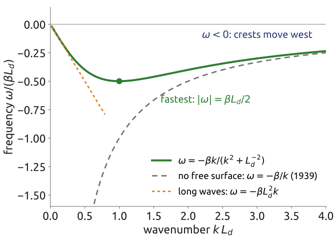
With a free surface and no wind, linearize the shallow-water potential vorticity about rest on the beta-plane, for \(|\eta| \ll H\) and \(|\zeta| \ll f_0\): \[ Q = \frac{\zeta + f_0 + \beta y}{H + \eta} \approx \frac{1}{H}\left(f_0 + \beta y + \zeta - \frac{f_0\,\eta}{H}\right) . \] Its conservation, linearized (the advection by \(\mathbf{u}\) of the perturbation is quadratic and dropped, the advection of \(\beta y\) is \(\beta v\)), reads \(\partial_t(\zeta - f_0\eta/H) + \beta v = 0\). For slow motions the velocity is geostrophic, given by the streamfunction \(\psi = g\eta/f_0\): \(u = -\partial_y\psi\), \(v = \partial_x\psi\), \(\zeta = \nabla^2\psi\), and \(f_0\eta/H = f_0^2\psi/(gH) = \psi/L_d^2\). Hence \[ \frac{\partial}{\partial t}\left(\nabla^2\psi - \frac{\psi}{L_d^2}\right) + \beta\,\frac{\partial\psi}{\partial x} = 0 , \] and for \(\psi \propto e^{i(kx + ly - \omega t)}\), \(-i\omega\,(-k^2 - l^2 - L_d^{-2}) + i\beta k = 0\), that is (Vallis 2017, sec. 6.4.2, eq. 6.65 with no mean flow) \[ \omega = -\frac{\beta k}{k^2 + l^2 + L_d^{-2}} . \tag{14}\] The phase always moves west, \(\omega/k < 0\). The waves are slow: the largest frequency, at \(k = 1/L_d\) and \(l = 0\), is \(\beta L_d/2\) (Figure 36), which gives periods of at least 9 days in the atmosphere (\(L_d = NH/f \approx 1000\) km).
Short waves, \(K \gg 1/L_d\), have \(\omega = -\beta k/K^2\), Equation 13 without wind: the case Rossby studied (Rossby and collaborators 1939). With a free surface and a wind together, the wind also tilts the surface and changes the potential-vorticity gradient to \(\beta + U/L_d^2\), so it is no longer a pure shift of the frequency (Vallis 2017, eqs. 6.66–6.68); the barotropic case keeps the picture simple. The stationary wavelength \(2\pi\sqrt{U/\beta}\) is about 6000 km at \(45^\circ\)N for \(U = 15\) m/s: four or five of them fit around the latitude circle, as the large troughs and ridges of the upper-level flow. Long waves, \(K \ll 1/L_d\), all travel west at the same speed \(\beta L_d^2\). In the ocean, with an internal \(L_d\) of some tens of kilometres, this is a few centimetres per second: these waves take years to cross an ocean basin, and satellite altimeters see them (Chelton and Schlax 1996).
38 Rossby waves (3/4): reading the diagram
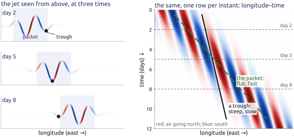
A longitude–time diagram, or Hovmöller diagram (Hovmöller 1949), follows a quantity along a latitude circle in time: each row is the line at one instant, and time runs down (Figure 37). Something that stands still draws a vertical stripe; something moving east draws a stripe tilted to the right, the flatter the faster, and its speed is the slope, distance over time. On the jet the natural quantity is the northward wind \(v\): red where the air goes north, blue where it goes south, so that going east a change from blue to red marks a trough, where the jet dips towards the equator: a trough is a low-pressure system, and at its bottom the air moves neither north nor south, so it lies on the white boundary between the two colours.
A Rossby wave packet then shows two slopes. The troughs and ridges, the phase, move slowly, at \(\omega/k\); the packet, the region where the meanders are large, moves at the group velocity \(c_g\), faster east (Equation 13 and after). So each trough grows as the packet reaches it and fades when the packet has passed, while new troughs grow ahead of the packet: what travels fast is the pattern of growing waves, sometimes called downstream development.
39 Rossby waves (4/4): theory against data
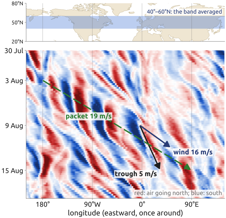
The Rossby wave packet of early August 2002, which crossed the northern hemisphere before the Elbe flood (Wirth et al. 2018), shows the three speeds of Equation 13 (Figure 38). Figure 38 is a longitude–time diagram of the northward wind at 250 hPa, near the jet, averaged from \(40^\circ\) to \(60^\circ\)N (ERA5, (Hersbach et al. 2020)). From 3 to 15 August the mean eastward wind there was 16 m/s at 250 hPa and 8 m/s at 500 hPa. The troughs crawled east, slower than the wind: the one that reached western Europe went from \(4^\circ\)W on 9 August to \(33^\circ\)E on 15 August, about 5 m/s, and all troughs together moved at about 3 m/s (lagged correlation of the field filtered to zonal wavenumbers 4–10). The packet, the region of large waves, ran east much faster: from \(180^\circ\) on 3 August to \(90^\circ\)E on 15 August, about 19 m/s (Wirth et al. 2018, 1972).
In the barotropic theory with \(l = 0\), the dominant zonal wavenumber 6 at \(50^\circ\)N (a wavelength of 4300 km) has \(\beta/k^2 \approx 7\) m/s. With the wind at 500 hPa the theory gives troughs at 1 m/s and a packet at 15 m/s; with the wind at 250 hPa, 9 and 22 m/s. The data fall between the two: the waves are steered by the wind of the whole troposphere, not of one level. The theory is rough (it ignores the jet’s own potential-vorticity gradient and the vertical structure of the waves), but the order is right: troughs slower than the wind, the packet faster than both.
40 Fast and slow: the four waves
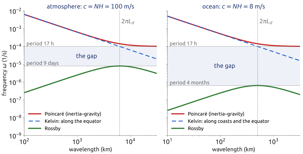
The four waves of rotating shallow water, gravity waves (without rotation), Poincaré, Kelvin and Rossby waves, fall into two families separated by a gap (Figure 39). The fast ones are the Poincaré (inertia–gravity) waves, with frequencies above \(f\), periods below \(2\pi/f\) (17 h at \(45^\circ\)N), and the Kelvin waves, which travel at the gravity-wave speed \(c\). The slow ones are the Rossby waves, with frequencies below \(\beta L_d/2\): periods of more than 9 days in the atmosphere, more than 4 months in the ocean, whose internal deformation radius is ten times smaller. Kelvin waves, with \(\omega = ck\), exist at any frequency, also in the gap, but only along a wall: in the atmosphere the equator, in the ocean the coasts and the equator. Balance lives below the gap: the weather and the ocean currents are slow, near the geostrophic mode and in the Rossby branch (Vallis 2017, sec. 3.8, §6.4; Gill 1982). The fast waves carry little of the weather, but in a model they set the time step: an explicit time step must resolve the fastest wave, and the fast branch is ten to a hundred times faster than the slow one.
41 Geostrophic adjustment (1/3): release a step
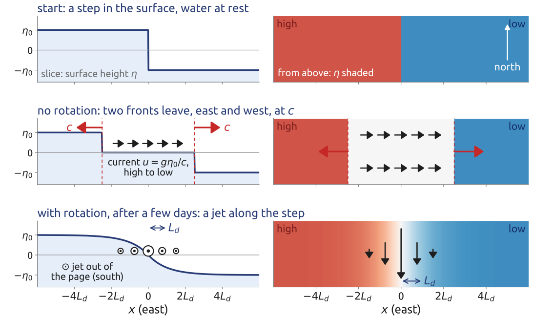
How does a fluid reach geostrophic balance? Rossby answered with the simplest unbalanced state: a step in the surface, \(\eta = +\eta_0\) for \(x < 0\) and \(\eta = -\eta_0\) for \(x > 0\), with the fluid at rest, in the linear equations Equation 8 on the f-plane, independent of \(y\) (Rossby 1938; Vallis 2017, sec. 3.9, eq. 3.137). At the start the pressure pushes from high to low, and nothing balances it. With no change in \(y\) the equations are (Vallis 2017, eqs. 3.136a,b) \[ \frac{\partial u}{\partial t} - fv = -g\frac{\partial\eta}{\partial x}, \qquad \frac{\partial v}{\partial t} = -fu, \qquad \frac{\partial\eta}{\partial t} + H\frac{\partial u}{\partial x} = 0 . \]
Without rotation, the equations reduce to the wave equation in \(x\), whose solution is the initial shape carried left and right at speed \(c\) (Vallis 2017, sec. 3.9.1, eqs. 3.139–3.142): \[ \eta(x, t) = -\frac{\eta_0}{2}\big[\mathrm{sgn}(x + ct) + \mathrm{sgn}(x - ct)\big] , \] with \(\mathrm{sgn}\) the sign function. Two fronts leave at speed \(c\), like the waves of a dam break. Behind them the surface is flat, \(\eta = 0\), and the water flows uniformly at \(u = g\eta_0/c\) from the high side to the low side (Figure 40). The step is gone, carried away by gravity waves; for a finite bump (a “top hat”), the fronts of its two edges pass and leave the fluid at rest and flat: nothing is left.
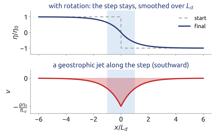
With rotation, the second equation, \(\partial v/\partial t = -fu\), turns the current that crosses the step into a current along it, until \(fv = g\,\partial\eta/\partial x\): the flow becomes geostrophic, and the Coriolis force on the current along the step balances the slope. Part of the step stays (Figure 40); how much, the next section computes from potential vorticity. The adjustment also leaves inertial oscillations, which decay slowly.
42 Geostrophic adjustment (2/3): what is kept
With rotation, one quantity does not change while the waves sort the flow out. From the equations of Section 41, with \(f = f_0\), take \(\partial/\partial x\) of the second, \(\partial v/\partial t = -f_0u\): with \(\zeta = \partial v/\partial x\), \(\partial\zeta/\partial t = -f_0\,\partial u/\partial x\). The third gives \(\partial u/\partial x = -H^{-1}\,\partial\eta/\partial t\). Put together, \[ \frac{\partial q}{\partial t} = 0, \qquad q = \zeta - \frac{f_0\,\eta}{H} , \] the linear potential vorticity (Vallis 2017, sec. 3.9.2, eqs. 3.143–3.146). It is the linear form of the \((\zeta + f)/h\) kept by each column: \(Q = (\zeta + f_0)/(H + \eta) \approx (f_0 + q)/H\), and its advection, a product of small quantities, is dropped, so \(q\) is fixed not only following the fluid but at each point. At the start \(\zeta = 0\) and \(\eta = -\eta_0\,\mathrm{sgn}(x)\), so \[ q(x) = \frac{f_0\eta_0}{H}\,\mathrm{sgn}(x) \] for ever, whatever the waves do (Figure 41). Without rotation \(q = \zeta = 0\) is kept too, but it says nothing about \(\eta\); with \(f_0\) it ties the final \(\eta\) to the initial one.
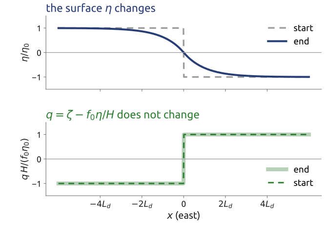
43 Geostrophic adjustment (3/3): the balanced state
If the fluid settles into a steady state, that state is geostrophic, \(f_0 v = g\,\partial\eta/\partial x\), \(u = 0\), and has the same \(q\). Then \(\zeta = \partial v/\partial x = (g/f_0)\,\partial^2\eta/\partial x^2\), and \(q = \zeta - f_0\eta/H\) becomes, multiplied by \(f_0/g\) and with \(L_d^2 = gH/f_0^2\), \[ \frac{\partial^2\eta}{\partial x^2} - \frac{\eta}{L_d^2} = \frac{\eta_0}{L_d^2}\,\mathrm{sgn}(x) . \] Vallis writes the same equation for the streamfunction \(\psi = g\eta/f_0\), \(\partial^2\psi/\partial x^2 - \psi/L_d^2 = q\) (Vallis 2017, eqs. 3.148–3.149). Solve on each side, with \(\eta\) and \(\partial_x\eta\) continuous at \(x = 0\) and \(v \to 0\) far away: \[ \eta = -\eta_0\,\mathrm{sgn}(x)\left(1 - e^{-|x|/L_d}\right), \qquad v = -\frac{g\eta_0}{f_0L_d}\,e^{-|x|/L_d} . \] The step stays, smoothed over a distance \(L_d\), with a geostrophic jet along it (Figure 42). Potential vorticity and geostrophy alone give the final state, without following the waves.
Energy. Per unit length in \(y\) and per unit density, the potential energy released is \(\frac{g}{2}\int(\eta_0^2 - \eta^2)\,dx = \frac{3}{2}\,g\eta_0^2L_d\), and the kinetic energy of the jet is \(\frac{H}{2}\int v^2\,dx = \frac{1}{2}\,g\eta_0^2L_d\) (using \(gH/f_0^2 = L_d^2\)). Only one third of the energy released stays in the balanced flow; two thirds are carried away by Poincaré waves (Vallis 2017, sec. 3.9.3; Gill 1982, sec. 7.2). Rotating fluids adjust to balance by radiating gravity waves: this is why the large-scale flow is nearly geostrophic. It is also why an unbalanced initial state, such as the one of Richardson’s forecast, fills a model with spurious gravity waves.
44 Adjustment computed: fronts that leave, a step that stays
Which speed \(c\) to use depends on what moves. If the whole depth moves together, the external mode, \(c = \sqrt{gH}\): about 300 m/s for a 10 km atmosphere and 200 m/s for a 4 km ocean, with deformation radii of thousands of kilometres. Inside a stratified fluid gravity is weak: its internal gravity waves travel at about \(NH\), and the first vertical mode, in which the upper and lower parts move in opposite directions, at \(c_1 = NH/\pi\) for a constant buoyancy frequency \(N\) (Vallis 2017, sec. 3.4.2, eq. 3.67): about 32 m/s in the troposphere and 2.5 m/s in the ocean (Figure 43). Both modes have the same inertial bound for the Poincaré waves, but the slow Rossby waves of the internal mode are much slower, and its deformation radius much smaller: the stratification makes the small, slow motions of weather and of ocean eddies.
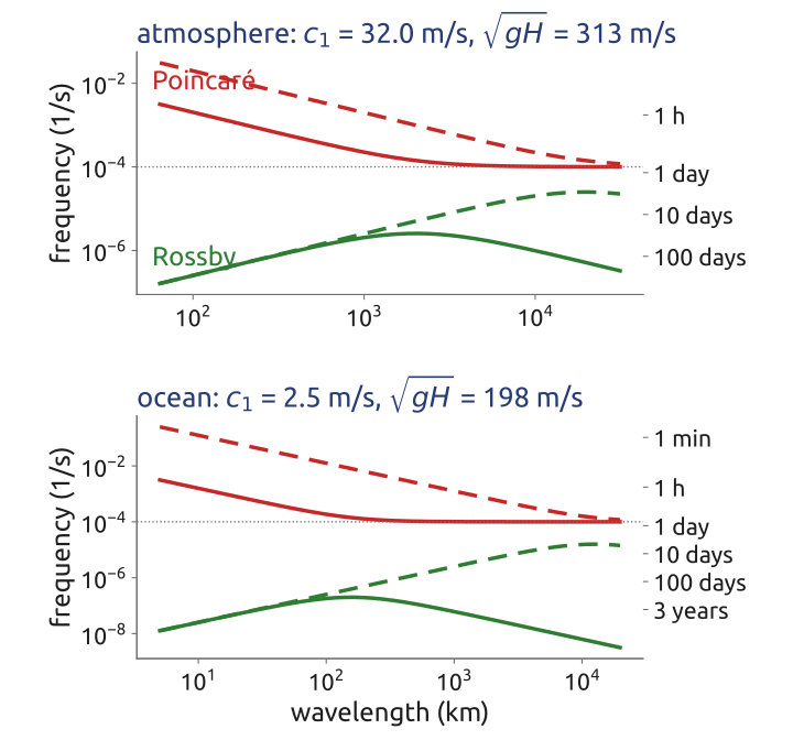
The same problem can be solved numerically with the linear equations Equation 8, from the step at rest to the end of the adjustment, here with \(H = 100\) m, \(f = 10^{-4}\) s\(^{-1}\), so \(c = 31\) m/s and \(L_d = 313\) km (Figure 44). Two gravity-wave fronts leave at speed \(c\); between them the surface settles on the balanced profile of Section 43, while inertial oscillations, of period \(2\pi/f\), slowly decay. A time–distance (Hovmöller) diagram shows both at once: what leaves travels along the lines \(x = \pm ct\), what stays does not move. The kinetic energy of the final jet, compared with the potential energy released, is the one third of Section 43.
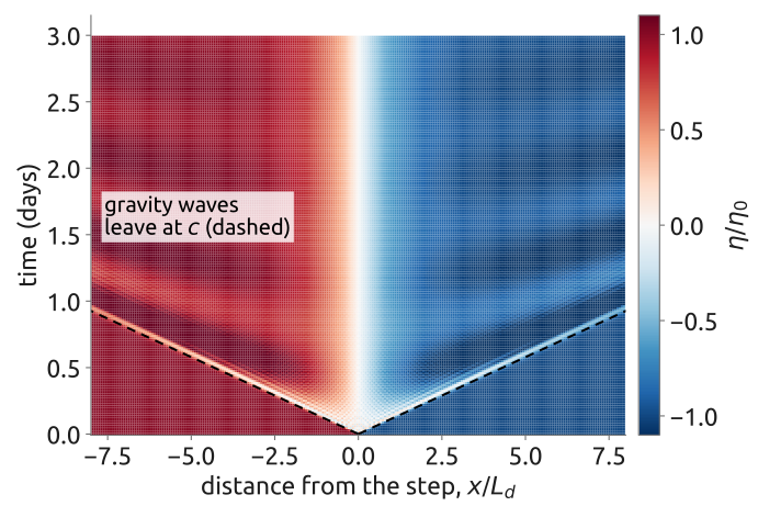
45 Narrow bumps leave, wide bumps stay
How the step adjusts, in time (Figure 45): at the start only the pressure acts, and the water runs from high to low, across the step (\(u > 0\) with the high to the west), while two gravity-wave fronts leave at \(c\). The Coriolis force turns this current to its right, along the step (\(v < 0\), southward): within about half an inertial period, \(\pi/f \approx 9\) h, most of \(u\) has become \(v\). The turn overshoots; what is left of the imbalance oscillates at the inertial period \(2\pi/f\) and slowly decays, and after a few days \(v\) is Rossby’s jet, within \(L_d\) of the step. A step that is sharp on the grid adds ripples behind the fronts, at any resolution, because the shortest waves travel too slowly on the grid; a step smoothed over a few grid cells avoids them.
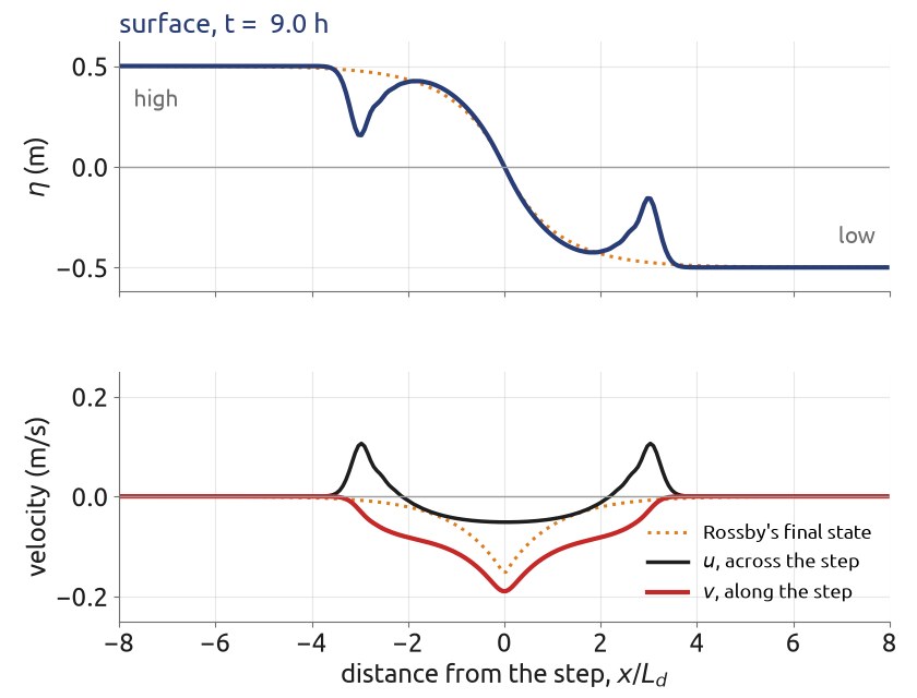
Release a bump of the surface at rest instead of a step (Figure 46). Without rotation it splits into two gravity waves travelling at \(\sqrt{gH}\), and nothing stays. With rotation part of it stays: a hill of width about \(L_d\), in geostrophic balance, while Poincaré waves leave. How much stays depends on the width \(R\) of the bump. Its linear potential vorticity, \(q = -f_0\eta/H\) at the start, stays where it is, and the final state is its inversion, \(\partial_x^2\psi - \psi/L_d^2 = q\). A wide bump, \(R \gg L_d\), has \(\partial_x^2\psi \ll \psi/L_d^2\), so \(\psi \approx -L_d^2 q\), that is \(\eta\) unchanged: it is already balanced and stays. A narrow bump, \(R \ll L_d\), has its potential vorticity spread by the inversion over a width \(L_d\): in one dimension the remnant is a low, wide hill, of height about \(R/L_d\) times that of the bump, and most of the bump leaves as waves. For the step, the final state is Rossby’s solution, and its jet holds one third of the energy released.
Large-scale disturbances therefore stay balanced, while small ones are shaken off as waves. The atmosphere is forced at large scales, by heating, and stays near balance. In weather prediction the initial data must be balanced, or the model makes spurious gravity waves; removing them is the initialization of a forecast (Cushman-Roisin and Beckers 2011, sec. 15.2).
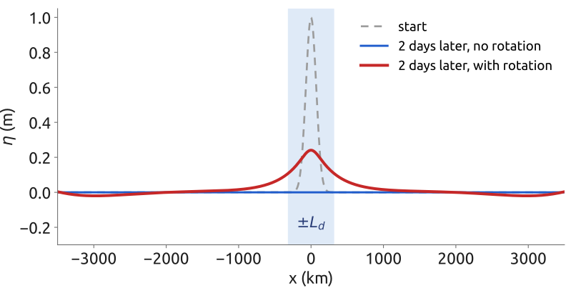
46 Quasi-geostrophy (1/2): from shallow water
Adjustment showed that the slow flow is geostrophic; the Rossby waves showed that it is carried by the potential vorticity. Charney turned this into equations without the fast waves (Charney 1948). Start from the shallow water equations with a flat bottom, \(h = H + \eta\), on the beta-plane, \(f = f_0 + \beta y\), written as the vorticity equation and the mass equation (the vorticity section above): \[ \frac{D(\zeta + f)}{Dt} = -(\zeta + f)\,\nabla\cdot\mathbf{u}, \qquad \frac{D\eta}{Dt} = -(H + \eta)\,\nabla\cdot\mathbf{u} . \] Assume that the Rossby number \(Ro = U/(f_0L)\) is small, that the scales are near the deformation radius, so that the surface displacement is small, \(\eta/H \sim Ro\,L^2/L_d^2\), and that \(f\) changes little over the flow, \(\beta L \ll f_0\) (Vallis 2017, sec. 5.3, assumptions (i)–(iv)). Then, order by order in \(Ro\) (Vallis 2017, sec. 5.3.1, eqs. 5.56–5.69; Cushman-Roisin and Beckers 2011, Ch. 16):
- Leading order: geostrophic. \(f_0\mathbf{k}\times\mathbf{u} = -g\nabla\eta\), so the velocity has no divergence and a streamfunction, \(\mathbf{u}_g = \mathbf{k}\times\nabla\psi = (-\partial_y\psi, \partial_x\psi)\) with \(\psi = g\eta/f_0\), and \(\zeta = \nabla^2\psi\).
- Vorticity at the next order. The divergence is a factor \(Ro\) smaller, and only the planetary vorticity is stretched (stretching by \(\zeta\) is smaller again by \(Ro\)): \(D_g(\zeta + \beta y)/Dt = -f_0\,\nabla\cdot\mathbf{u}\), with \(D_g/Dt = \partial_t + \mathbf{u}_g\cdot\nabla\), the derivative following the geostrophic flow.
- Mass eliminates the divergence. With \(\eta \ll H\), \(\nabla\cdot\mathbf{u} = -H^{-1}D_g\eta/Dt\), and so \(D_g(\zeta + \beta y - f_0\eta/H)/Dt = 0\).
With \(\zeta = \nabla^2\psi\) and \(f_0\eta/H = f_0^2\psi/(gH) = \psi/L_d^2\), \[ \frac{\partial q}{\partial t} + J(\psi, q) = 0, \qquad q = \nabla^2\psi - \frac{\psi}{L_d^2} + \beta y , \tag{15}\] the quasi-geostrophic potential vorticity equation. Here \[ J(a, b) = \frac{\partial a}{\partial x}\frac{\partial b}{\partial y} - \frac{\partial a}{\partial y}\frac{\partial b}{\partial x} \] is the Jacobian of two fields \(a\) and \(b\); with \(\mathbf{u}_g = (-\partial_y\psi, \partial_x\psi)\), \(\mathbf{u}_g\cdot\nabla q = J(\psi, q)\): the advection of \(q\) by the geostrophic flow. The order matters: \(J(q, \psi) = -J(\psi, q)\). The flow is geostrophic, but geostrophy alone does not make it evolve: it evolves through the small divergence that step 3 eliminates. And \(q\) is the shallow-water potential vorticity to first order: \(Q = (\zeta + f)/(H + \eta) \approx (f_0 + q)/H\), the \(q\) of the adjustment problem plus \(\beta y\).
47 Quasi-geostrophy (2/2): properties and practice
The equation has one unknown, \(\psi\), and one evolving field, \(q\). Each time step inverts \(q\) for \(\psi\) by solving the elliptic (Helmholtz) problem \[ \left(\nabla^2 - \frac{1}{L_d^2}\right)\psi = q - \beta y , \] and then advects \(q\) with the geostrophic velocity. The deformation radius sets how far the flow of a potential-vorticity anomaly reaches (Figure 47): with a free surface the flow is confined to a few \(L_d\).
The surface height is tied to the flow by geostrophy, so the gravity waves are gone; linearized about rest the equation gives the Rossby waves Equation 14, and nothing else. The time step of a model is then limited by the wind, \(U\), not by the gravity-wave speed \(c\), and can be ten times longer or more. The equation conserves the energy \[ E = \frac{1}{2}\int\left(|\nabla\psi|^2 + \frac{\psi^2}{L_d^2}\right)dA , \] kinetic plus potential (multiply Equation 15 by \(-\psi\) and integrate; the stratified form is Vallis (2017, sec. 5.6, eq. 5.159)), and the enstrophy \(\frac{1}{2}\int q^2\,dA\) (multiply by \(q\)), an invariant that appears only in the quasi-geostrophic limit (Vallis 2017, sec. 5.3.3). At a scale \(L\) the ratio of kinetic to potential energy is about \(L_d^2/L^2\): below \(L_d\) the energy is mostly kinetic, above it mostly potential.
It holds for small Rossby numbers, scales near \(L_d\) and small changes of \(f\): not near the equator, where \(f\) vanishes, and not at fronts, where the Rossby number is not small. Charney derived the same approximation for the continuously stratified atmosphere (Charney 1948); quasi-geostrophic models followed the first computer forecasts within a few years, and the primitive equations became operational only in the 1960s (Lynch 2008b). Today quasi-geostrophy is the language of much of the theory, and of idealized models of the atmosphere and the ocean. Its limit \(L_d \to \infty\), with no free surface, is the barotropic vorticity equation of the 1950 forecast.
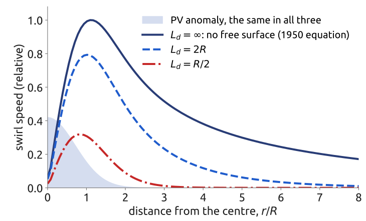
48 Barotropic vorticity (1/2): no divergence
The barotropic vorticity equation follows directly from shallow water, in three steps. Start from the vorticity equation, \(D(\zeta + f)/Dt = -(\zeta + f)\,\nabla\cdot\mathbf{u}\).
- Rigid lid. With a flat bottom and a surface that does not move, the depth is constant, \(h = H\), and the mass equation Equation 7 gives \(\nabla\cdot\mathbf{u} = 0\). The surface hardly moves when the motion is smaller than the deformation radius: for a geostrophic flow of size \(L\), \(\eta \sim f_0UL/g\), so \(\eta/H \sim f_0UL/(gH) = Ro\,L^2/L_d^2\). For the atmosphere the external deformation radius is about 3000 km and weather systems have \(L \approx 1000\) km, so \(L^2/L_d^2 \approx 0.1\): the approximation is reasonable.
- Absolute vorticity kept. With no divergence there is no stretching: \(D(\zeta + f)/Dt = 0\), each column keeps its absolute vorticity, as in Rossby’s 1939 analysis (Rossby and collaborators 1939).
- Streamfunction. A non-divergent flow derives from a streamfunction \(\psi\) (Vallis 2017, sec. 3.1.3): \[ u = -\frac{\partial\psi}{\partial y}, \qquad v = \frac{\partial\psi}{\partial x}, \qquad \zeta = \nabla^2\psi , \] and \(\nabla\cdot\mathbf{u} = -\partial_x\partial_y\psi + \partial_y\partial_x\psi = 0\) automatically. The velocity is along the contours of \(\psi\), the streamlines (Figure 48), and the advection is a Jacobian, \(\mathbf{u}\cdot\nabla = J(\psi, \cdot)\).
Together, \(\partial_t\nabla^2\psi + J(\psi, \nabla^2\psi + f) = 0\): one equation for one unknown, \(\psi\). It needs no expansion in the Rossby number: under the rigid lid it is exact. It is also the quasi-geostrophic equation Equation 15 in the limit \(L_d \to \infty\), where the term \(\psi/L_d^2\) disappears (Vallis 2017, sec. 5.3); there \(\psi\) comes from geostrophy, here from the absence of divergence.
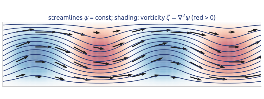
49 Barotropic vorticity (2/2): the 1950 forecast
With \(\mathbf{u} = \mathbf{k}\times\nabla\psi\), the advection is a Jacobian, \(\mathbf{u}\cdot\nabla(\zeta + f) = J(\psi, \zeta + f)\), and the conservation of \(\zeta + f\) becomes \[ \frac{\partial}{\partial t}\nabla^2\psi + J\big(\psi,\ \nabla^2\psi + f\big) = 0 , \tag{16}\] the barotropic vorticity equation, the limit \(L_d \to \infty\) of Equation 15. It has no surface height and no gravity waves; its only waves are Rossby waves, so its time step can be long. Each step has two parts: advance the vorticity \(\zeta = \nabla^2\psi\) in time, then recover \(\psi\), and with it the velocity, by solving the Poisson problem \(\nabla^2\psi = \zeta\).
This is the equation that Charney, Fjørtoft and von Neumann integrated on the ENIAC in 1950, for the flow at 500 hPa over North America, with 24-hour forecasts and time steps of up to three hours: the first successful computer forecast (Charney et al. 1950; Lynch 2008a) (Figure 49). Richardson’s forecast had kept the gravity waves, and an unbalanced initial state ruined it; the barotropic vorticity equation is shallow water with the fast waves filtered out.
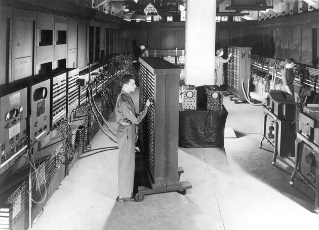

50 Ekman layer (1/4): friction near the surface
Geostrophic balance is the Coriolis force against the pressure force. Under the wind, near the sea surface, a third force takes part: friction. The simplest case, the Coriolis force against friction alone, is the Ekman layer, the answer of Ekman (1905) to Nansen’s question of why the Arctic ice drifted to the right of the wind. The same layer exists at the bottom of the ocean and at the bottom of the atmosphere. The derivation follows Cushman-Roisin and Beckers (2011, secs. 8.2, 8.6) and Vallis (2017, sec. 5.7).
Take a deep ocean of constant density \(\rho_0\) on the f-plane, in the northern hemisphere (\(f > 0\)), under a wind stress \(\boldsymbol{\tau} = (\tau_x, \tau_y)\), uniform and steady: the force per unit area (N/m\(^2\)) that the wind exerts on the sea surface, typically 0.1 N/m\(^2\). Look for a steady flow \(\mathbf{u}(z)\) that depends on depth only. There are then no horizontal gradients: the advection vanishes, continuity gives \(\partial w/\partial z = 0\) and so \(w = 0\), and the pressure exerts no horizontal force. Left are the Coriolis force and friction. Molecular friction is negligible, but the turbulence near the surface carries momentum up and down far better than the molecules do. The simplest model is an eddy viscosity \(\nu_E\), about \(10^{-2}\) m\(^2\)/s for the upper ocean, \(10^4\) times the molecular viscosity of water (Cushman-Roisin and Beckers 2011, sec. 8.2). The water above a horizontal surface pulls the water below with the stress \(\rho_0\nu_E\,\partial\mathbf{u}/\partial z\); a slab between \(z\) and \(z + \delta z\) feels this stress on its top face and the opposite one on its bottom face, a net force \(\rho_0\nu_E(\partial_z\mathbf{u}|_{z+\delta z} - \partial_z\mathbf{u}|_z) \approx \rho_0\nu_E\,\partial_z^2\mathbf{u}\,\delta z\) per unit area, that is \(\nu_E\,\partial^2\mathbf{u}/\partial z^2\) per unit mass. In a steady state it balances the Coriolis force (Figure 50): \[ f\,\mathbf{k}\times\mathbf{u} = \nu_E\,\frac{\partial^2\mathbf{u}}{\partial z^2}, \qquad\text{that is}\qquad -fv = \nu_E\,\frac{d^2u}{dz^2}, \quad fu = \nu_E\,\frac{d^2v}{dz^2} , \tag{17}\] with two boundary conditions: at the surface the stress in the water is the wind stress, and deep down the water is at rest, \[ \rho_0\nu_E\,\frac{d\mathbf{u}}{dz} = \boldsymbol{\tau} \quad\text{at } z = 0, \qquad \mathbf{u} \to 0 \quad\text{as } z \to -\infty . \tag{18}\] The net friction on a slab is at right angles to its velocity, to its left in the northern hemisphere, not against it, because it must cancel the Coriolis force.
Why only a thin layer. Over the whole depth \(H\) of the ocean the ratio of the two terms of Equation 17 is the Ekman number \[ Ek = \frac{\nu_E}{fH^2} \] (Vallis 2017, eq. 5.181; Cushman-Roisin and Beckers 2011, eq. 8.11), about \(10^{-5}\) (\(6\times10^{-6}\) for \(\nu_E = 10^{-2}\) m\(^2\)/s, \(f = 10^{-4}\) s\(^{-1}\) and \(H = 4\) km): friction is negligible in the interior. But friction is the term with the highest derivative: without it, Equation 17 is algebraic and cannot meet the surface condition. As in Prandtl’s boundary layers, friction survives in a thin layer where the shear is strong, of a thickness at which the local Ekman number is of order one, \(\sqrt{\nu_E/f} = H\,Ek^{1/2}\) (Vallis 2017, eqs. 5.185–5.186). The solution fixes the factor: the Ekman depth (Cushman-Roisin and Beckers 2011, eq. 8.16) \[ d = \sqrt{\frac{2\nu_E}{f}} , \] 14 m for \(\nu_E = 10^{-2}\) m\(^2\)/s. The eddy viscosity is a property of the turbulence, not of the water, and estimates vary: Vallis quotes about 0.1 m\(^2\)/s and Ekman depths of 50 m or less for the ocean, and about \(10^2\) m\(^2\)/s for the atmosphere, whose Ekman layer is about 1 km deep (Vallis 2017, sec. 5.7.1).
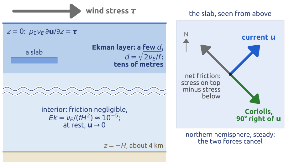
51 Ekman layer (2/4): one complex equation
Write the horizontal velocity as one complex number, with east as the real axis and north as the imaginary axis (Figure 51): \[ W = u + iv . \] Since \(\mathbf{k}\times\mathbf{u} = (-v, u)\) and \(iW = -v + iu\), the cross product with \(\mathbf{k}\) is the multiplication by \(i\), a rotation by \(90^\circ\) anticlockwise; more generally, multiplying by \(e^{-i\theta}\) turns a vector by \(\theta\) clockwise. The real and imaginary parts of \[ \nu_E\,\frac{d^2W}{dz^2} = if\,W \tag{19}\] are the two equations Equation 17. It is linear with constant coefficients: try \(W = A\,e^{\lambda z}\), with \(A\) a complex constant. Then \(\nu_E\lambda^2 = if\), so \(\lambda^2 = if/\nu_E = 2i/d^2\). Since \((1 + i)^2 = 1 + 2i - 1 = 2i\), \(\lambda = \pm(1 + i)/d\). The ocean lies below the surface, \(z < 0\), and \(e^{\lambda z}\) decays as \(z \to -\infty\) only if the real part of \(\lambda\) is positive. Hence \[ W(z) = A\,e^{(1+i)z/d} = A\,e^{z/d}\,e^{iz/d} . \] Each step \(d\) down, the current becomes \(e\) times weaker (\(e^{z/d}\)) and turns by one radian, \(57^\circ\) (\(e^{iz/d}\)): clockwise seen from above, since the argument \(z/d\) decreases with depth. In the southern hemisphere, \(f < 0\): with \(d = \sqrt{2\nu_E/|f|}\), the decaying root is \(\lambda = (1 - i)/d\) and the current turns anticlockwise. The complex form is that of Holton (2004, sec. 5.3.4, eqs. 5.29–5.31). Solved in real form, the pair Equation 17 gives the characteristic equation \(\nu_E^2\lambda^4 + f^2 = 0\), with the four roots \(\pm(1 \pm i)/d\), two of them decaying downwards (Cushman-Roisin and Beckers 2011, sec. 8.3, eq. 8.16).
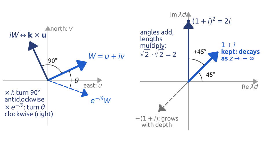
52 Ekman layer (3/4): the surface condition, 45°
Write the wind stress as a complex number too, \(\tau = \tau_x + i\tau_y\). The surface condition Equation 18 is \(\rho_0\nu_E\,W'(0) = \tau\), with \(W' = dW/dz\), and \(W'(0) = (1 + i)A/d\), so \[ A = \frac{\tau d}{\rho_0\nu_E(1 + i)} = \frac{\tau d\,(1 - i)}{2\rho_0\nu_E} = \frac{\sqrt{2}\,\tau}{\rho_0 fd}\,e^{-i\pi/4} , \] using \(\nu_E = fd^2/2\) and \(1 - i = \sqrt{2}\,e^{-i\pi/4}\). The solution is \[ W(z) = \frac{\sqrt{2}\,\tau}{\rho_0 fd}\,e^{z/d}\,e^{i(z/d - \pi/4)} , \] or, in real form (Cushman-Roisin and Beckers 2011, eq. 8.33; Vallis 2017, eqs. 5.213–5.214, without the geostrophic part), \[ \begin{aligned} u &= \frac{\sqrt{2}}{\rho_0 fd}\,e^{z/d}\left[\tau_x\cos\left(\frac{z}{d} - \frac{\pi}{4}\right) - \tau_y\sin\left(\frac{z}{d} - \frac{\pi}{4}\right)\right],\\ v &= \frac{\sqrt{2}}{\rho_0 fd}\,e^{z/d}\left[\tau_x\sin\left(\frac{z}{d} - \frac{\pi}{4}\right) + \tau_y\cos\left(\frac{z}{d} - \frac{\pi}{4}\right)\right]. \end{aligned} \] Three properties (Figure 52). (i) At the surface the current has the speed \(\sqrt{2}\,|\tau|/(\rho_0 fd)\), about 10 cm/s for \(|\tau| = 0.1\) N/m\(^2\), \(\rho_0 = 1025\) kg/m\(^3\) and \(d = 14\) m, and the factor \(e^{-i\pi/4}\) turns it \(45^\circ\) to the right of the wind in the northern hemisphere (to the left in the southern), whatever \(\nu_E\). (ii) Below, the current weakens as \(e^{z/d}\) and turns further to the right, by \(180^\circ\) every \(\pi d\): the tips of the current vectors, drawn from one point, trace the Ekman spiral, as Ekman drew it. At \(z = -\pi d\) the current is \(e^{-\pi} \approx 4\) % of the surface current and flows against it. (iii) At 10 m, for \(d = 14\) m, \(z/d = -0.7\): the water flows \(45^\circ + 41^\circ = 86^\circ\) to the right of the wind, almost across it, at half the surface speed.
The real ocean is less tidy. The eddy viscosity is not constant, and stratification makes the layer shallower. Observed angles between the near-surface current and the wind stress are well below \(45^\circ\), between about \(5^\circ\) and \(20^\circ\) (Cushman-Roisin and Beckers 2011, sec. 8.7), and clean spirals are rarely seen; current meters averaged over time have shown profiles broadly consistent with Ekman’s theory (Vallis 2017, sec. 5.7.5). What survives every refinement is the transport.
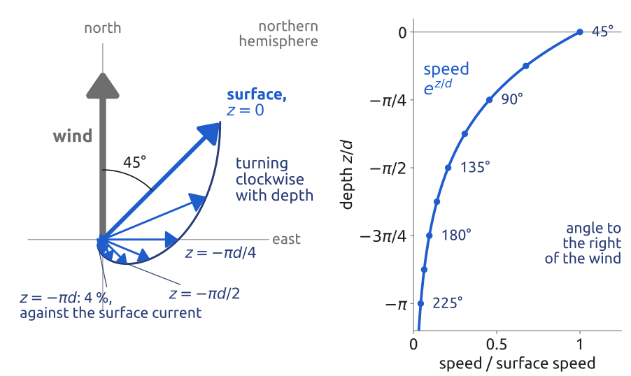
53 Ekman layer (4/4): transport and pumping
Integrate Equation 19 over the whole layer. With the transport \(M = \int_{-\infty}^0 W\,dz\), the volume transport per unit width (m\(^2\)/s), and \(W' \to 0\) deep down, \[ ifM = \nu_E\big[W'\big]_{-\infty}^{0} = \frac{\tau}{\rho_0} \qquad\Longrightarrow\qquad M = \frac{-i\tau}{\rho_0 f} . \] Multiplying by \(-i\) turns the stress by \(90^\circ\) clockwise: \(-iW\) corresponds to \(-\mathbf{k}\times\mathbf{u} = \mathbf{u}\times\mathbf{k}\). In vector form, \[ \mathbf{M}_E = \int_{-\infty}^{0}\mathbf{u}\,dz = \frac{\boldsymbol{\tau}\times\mathbf{k}}{\rho_0 f}, \qquad M_x = \frac{\tau_y}{\rho_0 f}, \quad M_y = -\frac{\tau_x}{\rho_0 f} \tag{20}\] (Cushman-Roisin and Beckers 2011, eq. 8.34, whose components are \((U, V)\); Vallis 2017, eq. 5.191a, whose \(\mathbf{M}_E\) is the mass transport, \(\rho_0\) times this one): \(90^\circ\) to the right of the wind in the northern hemisphere, to the left in the southern. The eddy viscosity has dropped out. In fact the result needs no model of the friction at all: integrating \(f\,\mathbf{k}\times\mathbf{u} = \rho_0^{-1}\,\partial\boldsymbol{\tau}/\partial z\), with any stress profile that falls from the wind stress at the surface to zero at the base of the layer, gives \(f\,\mathbf{k}\times\mathbf{M}_E = \boldsymbol{\tau}/\rho_0\) directly (Vallis 2017, sec. 5.7.2). Over the whole layer the friction between slabs cancels; only the wind stress at the top remains, and the Coriolis force on the total transport must balance it.
Where the wind stress varies in space, the transports of neighbouring places differ, and water piles up or is drawn away. Integrate the continuity equation \(\nabla\cdot\mathbf{u} + \partial w/\partial z = 0\) across the layer, from its base (a few \(d\) down, where the Ekman current has died out) to the surface, where \(w \approx 0\): \(0 - w_E = -\nabla\cdot\mathbf{M}_E\). The vertical velocity at the base of the layer is \[ w_E = \nabla\cdot\mathbf{M}_E = \mathbf{k}\cdot\nabla\times\left(\frac{\boldsymbol{\tau}}{\rho_0 f}\right) = \frac{\partial}{\partial x}\left(\frac{\tau_y}{\rho_0 f}\right) - \frac{\partial}{\partial y}\left(\frac{\tau_x}{\rho_0 f}\right) , \tag{21}\] using \(\nabla\cdot(\mathbf{A}\times\mathbf{k}) = \mathbf{k}\cdot\nabla\times\mathbf{A}\) for the constant vector \(\mathbf{k}\) (Cushman-Roisin and Beckers 2011, eq. 8.36; Vallis 2017, eq. 5.197). This is Ekman pumping: in the northern hemisphere a wind stress that turns clockwise (negative curl) pushes water down out of the layer, and one that turns anticlockwise draws water up. Over the subtropical North Atlantic (Figure 53) the trade winds blow westward near \(15^\circ\)N and the mid-latitude winds eastward near \(45^\circ\)N. The Ekman transport is northward under the trade winds and southward under the eastward winds: it converges in between, and water is pushed down. For a stress \(\tau_x = -\tau_0\cos(\pi y/L)\) with \(\tau_0 = 0.1\) N/m\(^2\) over \(L = 3300\) km and \(f = 7\times10^{-5}\) s\(^{-1}\) (at \(30^\circ\)N), \(|w_E| \approx \pi\tau_0/(\rho_0 fL) \approx 1.3\times10^{-6}\) m/s, some 40 m a year; \(10^{-6}\) m/s is the value usually taken for the subtropical gyres (Vallis 2017, sec. 20.5). Tiny, but it acts over whole ocean basins and for ever. The columns of the interior under the gyre are squashed from above: how they move is the question of Sverdrup’s theory.
The same balance holds at the bottom. Under a geostrophic flow over a flat bottom, friction brings the velocity to zero at the ground in a bottom Ekman layer, where the flow turns \(45^\circ\) to the left of the interior flow (northern hemisphere), towards low pressure (Cushman-Roisin and Beckers 2011, sec. 8.3; Vallis 2017, sec. 5.7.3). This is why the wind near the ground crosses the isobars towards low pressure, and why air converges into a cyclone near the ground; seen from the interior, the bottom Ekman layer acts as a linear drag that slowly spins the flow down (Vallis 2017, sec. 5.7.6).
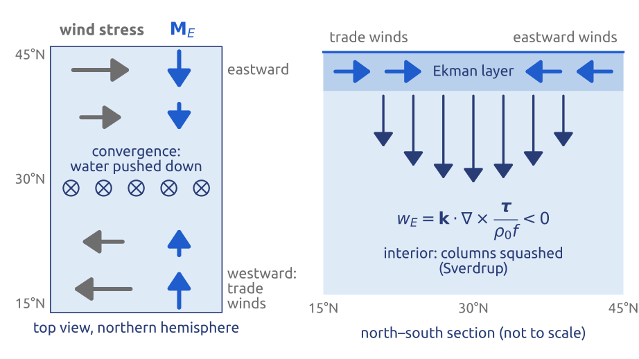
54 Sverdrup (1947): the wind drives the gyres
Start from the shallow water potential vorticity, now with forcing and friction: \(D[(\zeta + f)/h]/Dt = F/h\), with \(F\) the curl of the forces per unit mass, here the wind and friction (Vallis 2017, sec. 19.1.2, eq. 19.7). For an ocean with a rigid lid and a flat bottom, \(h = H\), this is the barotropic vorticity equation with a source [eq. 19.8]. The source is the curl of the wind stress, spread as a force over the depth \(H\), and a linear drag by the bottom Ekman layer, with a rate \(r\): \[ \frac{\partial\zeta}{\partial t} + J(\psi, \zeta) + \beta v = \frac{\mathbf{k}\cdot\nabla\times\boldsymbol{\tau}}{\rho_0 H} - r\zeta , \] with \(\psi\) the streamfunction, \(J(\psi, \zeta) = \mathbf{u}\cdot\nabla\zeta\) the advection of \(\zeta\), and \(\beta v = \mathbf{u}\cdot\nabla f\). For a steady, slow and wide flow, the advection of \(\zeta\) is small against \(\beta v\) (\(|\zeta| \ll \beta L\), that is \(U/(\beta L^2) \ll 1\)) and so is the friction (\(r\zeta \ll \beta v\)) (Vallis 2017, eqs. 19.11, 19.19). Only \(\beta v\) and the wind are left. With the northward transport per unit width \(V = Hv\), \[ \beta V = \frac{\mathbf{k}\cdot\nabla\times\boldsymbol{\tau}}{\rho_0} , \tag{22}\] the Sverdrup balance (Sverdrup 1947; Vallis 2017, sec. 19.1.3, eq. 19.20; Cushman-Roisin and Beckers 2011, sec. 20.2).
The columns explain it. In the subtropics of the northern hemisphere, Ekman pumping squashes the columns of the interior from above (Section 53); to keep \((\zeta + f)/h\) without spinning, they drift south, where \(f\) is smaller. The same balance follows by adding the two parts of the transport. Below the Ekman layer the flow is geostrophic, and its linear vorticity equation is \(\beta v = f\,\partial w/\partial z\): integrated from the flat bottom (\(w = 0\)) to the base of the Ekman layer (\(w = w_E\)), \(\beta V_g = f w_E\). The Ekman layer adds its own northward transport, \(-\tau_x/(\rho_0 f)\) by Equation 20, and with Equation 21 the sum is exactly Equation 22.
Numbers. A wind stress that changes by \(0.1\) N/m\(^2\) over 1000 km has a curl of about \(10^{-7}\) N/m\(^3\). At \(30^\circ\)N, \(\beta = 2\times10^{-11}\) m\(^{-1}\)s\(^{-1}\), so \(V \approx 10^{-7}/(10^3\times2\times10^{-11}) = 5\) m\(^2\)/s; across a basin 5000 km wide this is \(2.5\times10^7\) m\(^3\)/s, 25 Sv (\(1\ \text{Sv} = 10^6\) m\(^3\)/s), comparable with the transport of the Gulf Stream off Florida, about 30 Sv. The wind alone, through \(\beta\), sets the transport of the gyre.
The southward drift of the interior must return north somewhere. Stommel (1948) showed, with bottom friction, that the return flow is narrow and fast and lies on the western side of the basin, and that it is the variation of \(f\) with latitude that puts it there (Figure 54): this is why the Gulf Stream and the Kuroshio are western boundary currents. The same \(\beta\) that makes the Rossby waves travel west drives and shapes the ocean gyres.
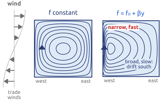
55 Key points
- Thin and slow: hydrostatic (\(\partial p/\partial z = -\rho g\)) and nearly geostrophic (\(Ro \ll 1\)).
- Shallow water: \(D\mathbf{u}/Dt + f\,\mathbf{k}\times\mathbf{u} = -g\nabla\eta\), \(\partial_t h + \nabla\cdot(h\mathbf{u}) = 0\); linear: Laplace’s tidal equations.
- Potential vorticity \((\zeta + f)/h\) is kept by each column: depth and latitude steer the flow.
- Waves: gravity, \(c = \sqrt{gH}\); Poincaré, \(\omega^2 = f^2 + c^2K^2\); Kelvin, trapped at coasts and at the equator, travelling one way only.
- Rossby waves: \(\omega/k = U - \beta/K^2\): carried east by the wind, drifting west through the air; the deformation radius is \(L_d = \sqrt{gH}/f\).
- Adjustment: imbalance leaves as gravity waves; what is wider than \(L_d\) stays, in geostrophic balance.
- Quasi-geostrophy: one potential vorticity, inverted for \(\psi\) at each step; with no divergence, the barotropic vorticity equation of the 1950 forecast.
- Ekman: friction makes a transport \(90^\circ\) to the right of the wind (northern hemisphere); its pumping, with \(\beta\), drives the ocean gyres (Sverdrup).
A thin rotating layer of fluid holds balance, potential vorticity and the waves of weather.
Further reading
Vallis (2017): §2.2–2.4 (spherical coordinates, the primitive equations, the tangent plane, the Boussinesq approximation), §2.7–2.8 (scaling, balance), Ch. 3 (shallow water, waves, adjustment), §3.7.1 and §4.5 (potential vorticity), §5.3 (quasi-geostrophy), §5.7 (the Ekman layer), §6.4 (Rossby waves), §8.2 (equatorial waves), §19.1 (the wind-driven gyres). Cushman-Roisin and Beckers (2011): Ch. 4, 7 and 9 (scales, shallow water and vorticity, barotropic waves), Ch. 8 (the Ekman layer), §15.2 (adjustment), Ch. 16 (quasi-geostrophy), §20.2–20.3 (Sverdrup balance and western boundary currents). Holton (2004): §2.4 (scale analysis), §4.3 (potential vorticity), §5.3 (the Ekman layer). Gill (1982), Ch. 7, for the adjustment problem in depth; Matsuno (1966) for the equatorial waves. For the mathematics: Azérad and Guillén (2001) on the hydrostatic limit, Majda (2003) for waves and balanced models. History: Richardson (1922), Ch. 4, for the equations as Richardson wrote them; Lynch (2008a) for the 1950 forecast.