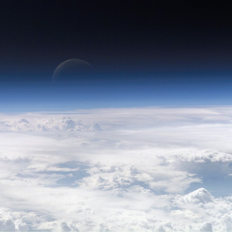
November 2026 · Politecnico di Milano

Reduced models: scales, balance, waves

Atmosphere and Ocean Dynamics — Lecture 3

Prof. Dr. Pedro da Silva Peixoto

Applied Mathematics
Instituto de Matemática e Estatística
Universidade de São Paulo

Visiting Professor at MOX Lab
Politecnico di Milano

Warm-up

1. A weather station sees the temperature fall, although every parcel keeps its temperature. Write the relation.
2. What does \(\nabla\cdot\mathbf{u}\) measure? A parcel with \(\nabla\cdot\mathbf{u} < 0\): does it get denser or lighter?
3. Where did the centrifugal force go in the momentum equation on the rotating Earth?

Title photo: NASA, ISS (2006), public domain, commons.wikimedia.org: Top of Atmosphere.jpg

Lecture 2, from memory: answer on paper first, 3 minutes (its carry-forward list).

1. dT/dt = -u . grad T (DT/Dt = 0). 2. The rate at which a parcel’s volume grows; denser.
2. Into the geopotential Phi, exactly; Phi = gz then takes the surfaces of constant Phi as spheres, an error of Omega^2 a/g = 3e-3 (the Earth is oblate).

Where we are and where we are going

Previous knowledge

• Seven equations, seven unknowns: momentum, \(\dfrac{D\mathbf{u}}{Dt} + 2\boldsymbol{\Omega}\times\mathbf{u} = -\dfrac{1}{\rho}\nabla p - \nabla\Phi + \mathbf{F}\), mass, gas law, first law
• Parcel or fixed point: \(DT/Dt = 0\) gives \(\partial T/\partial t = -\mathbf{u}\cdot\nabla T\)
• \(\nabla\cdot\mathbf{u} < 0\): the parcel’s volume shrinks, it gets denser
• The centrifugal force is inside the geopotential, \(\Phi \approx gz\)
• No heating: each parcel keeps its potential temperature \(\theta\)
• Sound and gravity waves (minutes to hours), slow weather (days)

Where we are going

1. Scales: hydrostatic, primitive equations
2. Shallow water, step by step
3. Vorticity and potential vorticity
4. Waves and the deformation radius \(L_d\)
5. Geostrophic adjustment, notebook
6. Quasi-geostrophy and the 1950 equation
7. The wind-driven ocean: Ekman, Sverdrup

Drop what is small, and the physics shows: balance, potential vorticity, waves

(Vallis 2017, Ch. 2–5; Cushman-Roisin and Beckers 2011, Ch. 4, 7, 9)

Two minutes. Left: what we take as known (lectures 1–2; the warm-up checked it). Right: the road of the day; each item links to its first slide. The next slide shows the same road as a ladder of models.

Today: keep the slow, large motions

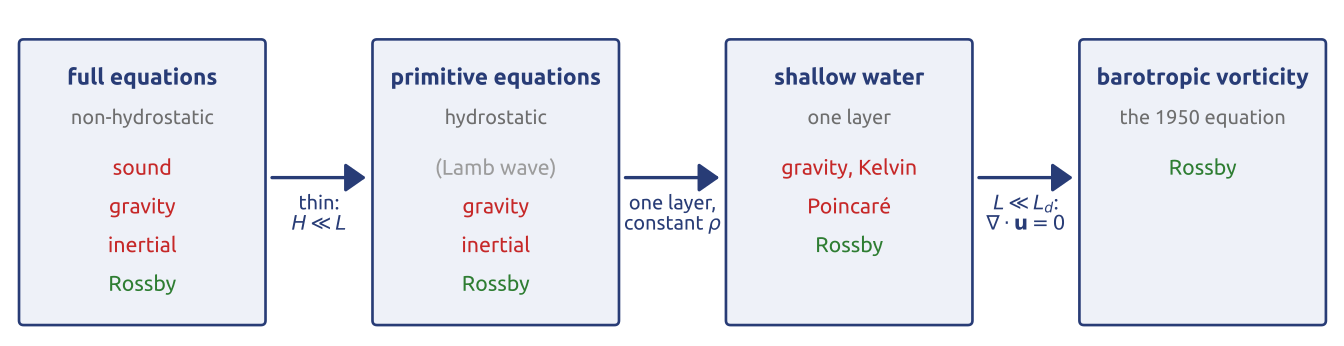
\(H\): depth of the fluid; \(L\): horizontal size of the motion; \(L_d = \sqrt{gH}/f\): deformation radius, the distance a gravity wave travels in a time \(1/f\)

• The full equations carry sound and gravity waves: Richardson’s 145 hPa in 6 hours

• Step by step, down to the 1950 forecast; each step keeps fewer waves: fast, slow

A ladder of models: each step drops terms that are small for large, slow motions

(Vallis 2017, Ch. 2–3; Charney 1948)

The plan of the day. Each box keeps fewer waves. Richardson: lecture 1. Shallow water is the workhorse of the numerics days (lectures 5, 6, 7, 8).

Scale analysis (1/4): the equations in components

\(\dfrac{D\mathbf{u}}{Dt} + 2\boldsymbol{\Omega}\times\mathbf{u} = -\dfrac{1}{\rho}\nabla p - \nabla\Phi + \mathbf{F}\) written out in local axes at latitude \(\varphi\): \(x\) east, \(y\) north, \(z\) up, on a sphere of radius \(a\):

\[\begin{aligned} \underbrace{\frac{Du}{Dt}}_{\text{acceleration}} \underbrace{-\,2\Omega v\sin\varphi + 2\Omega w\cos\varphi}_{\text{Coriolis}} \underbrace{+\,\frac{uw}{a} - \frac{uv\tan\varphi}{a}}_{\text{curvature}} &= \underbrace{-\frac{1}{\rho}\frac{\partial p}{\partial x}}_{\text{pressure}} \quad \underbrace{+\,F_x}_{\text{friction}}\\[4pt] \frac{Dv}{Dt} + 2\Omega u\sin\varphi + \frac{vw}{a} + \frac{u^2\tan\varphi}{a} &= -\frac{1}{\rho}\frac{\partial p}{\partial y} + F_y\\[4pt] \frac{Dw}{Dt} - 2\Omega u\cos\varphi - \frac{u^2 + v^2}{a} &= -\frac{1}{\rho}\frac{\partial p}{\partial z} - g + F_z \end{aligned}\]

\(u, v, w\): eastward, northward, upward velocity; \(\Omega\): rotation rate of the Earth; \(p\): pressure; \(\rho\): density; \(g\): gravity, with its centrifugal part; \(\mathbf{F} = \nu\nabla^2\mathbf{u}\): friction, \(\nu\): viscosity. Terms in \(1/a\): the axes turn as a parcel moves over the curved Earth

(Holton 2004, sec. 2.3, eqs. 2.19–2.21; Vallis 2017, sec. 2.2.3)

Holton’s form: local Cartesian axes on the sphere, metric terms kept. Do not derive the curvature terms on the board (Vallis 2.2); say where they come from: east and north change direction as the parcel moves.

Scale analysis (2/4): the size of each term

Typical sizes:

• \(U\), \(W\): horizontal and vertical speed
• \(L\): horizontal size; \(H\): depth
• Time \(L/U\): so \(D/Dt \sim U/L\)
• \(\delta P\): horizontal pressure change; \(P_0\): surface pressure
• \(f_0 = 2\Omega\sin\varphi_0\), \(\varphi_0\): central latitude; at \(45^\circ\), \(2\Omega\cos\varphi_0\) is as large

\[\begin{array}{cccccccc} \dfrac{Du}{Dt} & -\,2\Omega v\sin\varphi & +\,2\Omega w\cos\varphi & +\,\dfrac{uw}{a} & -\,\dfrac{uv\tan\varphi}{a} & = & -\dfrac{1}{\rho}\dfrac{\partial p}{\partial x} & +\,F_x\\[10pt] {\color{#1f5ccc}{\dfrac{U^2}{L}}} & {\color{#1f5ccc}{f_0U}} & {\color{#1f5ccc}{f_0W}} & {\color{#1f5ccc}{\dfrac{UW}{a}}} & {\color{#1f5ccc}{\dfrac{U^2}{a}}} & & {\color{#1f5ccc}{\dfrac{\delta P}{\rho L}}} & {\color{#1f5ccc}{\dfrac{\nu U}{H^2}}} \end{array}\]

\[\begin{array}{ccccccc} \dfrac{Dw}{Dt} & -\,2\Omega u\cos\varphi & -\,\dfrac{u^2 + v^2}{a} & = & -\dfrac{1}{\rho}\dfrac{\partial p}{\partial z} & -\,g & +\,F_z\\[10pt] {\color{#1f5ccc}{\dfrac{UW}{L}}} & {\color{#1f5ccc}{f_0U}} & {\color{#1f5ccc}{\dfrac{U^2}{a}}} & & {\color{#1f5ccc}{\dfrac{P_0}{\rho H}}} & {\color{#1f5ccc}{g}} & {\color{#1f5ccc}{\dfrac{\nu W}{H^2}}} \end{array}\]

Ratios: acceleration over Coriolis, \((U^2/L)/(f_0U) = U/(f_0L) = Ro\), the Rossby number; depth over size, \(H/L\), the aspect ratio.

Each term replaced by its size: put in the numbers, and the small terms show themselves

(Holton 2004, sec. 2.4, Tables 2.1–2.2; Vallis 2017, secs. 2.7.2, 2.8.1)

Ask first: which two terms of the x equation are largest for a weather system? The y equation scales the same way. Friction: molecular nu over the depth H (Holton); near the ground the shear is much larger (Ekman layer, later).

Scale analysis (3/4): the horizontal equations

A mid-latitude weather system (45°N): \(U = 10\) m/s, \(W = 1\) cm/s, \(L = 1000\) km, \(H = 10\) km,
\(\delta P = 10\) hPa, \(\rho \approx 1\) kg/m³, \(f_0 = 10^{-4}\ \mathrm{s^{-1}}\), \(a = 6400\) km, molecular \(\nu = 1.5\times10^{-5}\) m²/s

\[\begin{array}{cccccccc} \dfrac{Du}{Dt} & -\,2\Omega v\sin\varphi & +\,2\Omega w\cos\varphi & +\,\dfrac{uw}{a} & -\,\dfrac{uv\tan\varphi}{a} & = & -\dfrac{1}{\rho}\dfrac{\partial p}{\partial x} & +\,F_x\\[6pt] {\color{#1f5ccc}{\dfrac{U^2}{L}}} & {\color{#1f5ccc}{f_0U}} & {\color{#1f5ccc}{f_0W}} & {\color{#1f5ccc}{\dfrac{UW}{a}}} & {\color{#1f5ccc}{\dfrac{U^2}{a}}} & & {\color{#1f5ccc}{\dfrac{\delta P}{\rho L}}} & {\color{#1f5ccc}{\dfrac{\nu U}{H^2}}}\\[4pt] 10^{-4} & {\color{#c62828}{\mathbf{10^{-3}}}} & 10^{-6} & 10^{-8} & 10^{-5} & & {\color{#c62828}{\mathbf{10^{-3}}}} & 10^{-12}\\[2pt] {\color{#283c76}{\rule{1.8em}{2.40em}}} & {\color{#c62828}{\rule{1.8em}{2.60em}}} & {\color{#283c76}{\rule{1.8em}{2.00em}}} & {\color{#283c76}{\rule{1.8em}{1.60em}}} & {\color{#283c76}{\rule{1.8em}{2.20em}}} & & {\color{#c62828}{\rule{1.8em}{2.60em}}} & {\color{#6e6e6e}{\rule{1.8em}{0.80em}}} \end{array}\]

Bars: size of each term on a logarithmic scale, in m/s²

Geostrophic balance: Coriolis ≈ pressure force; the acceleration is \(Ro = 0.1\) of them

(Holton 2004, sec. 2.4, Table 2.1; Vallis 2017, sec. 2.8)

Holton’s Table 2.1, in m/s^2. Ask first: which two terms balance? The y equation gives the same. Geostrophic to about 10 %. Curvature, the f w term and uw/a are smaller still: dropped in the primitive equations.

Scale analysis (4/4): the vertical equation

The same weather system, with \(P_0 = 1000\) hPa at the ground and \(g \approx 10\) m/s²:

\[\begin{array}{ccccccc} \dfrac{Dw}{Dt} & -\,2\Omega u\cos\varphi & -\,\dfrac{u^2 + v^2}{a} & = & -\dfrac{1}{\rho}\dfrac{\partial p}{\partial z} & -\,g & +\,F_z\\[6pt] {\color{#1f5ccc}{\dfrac{UW}{L}}} & {\color{#1f5ccc}{f_0U}} & {\color{#1f5ccc}{\dfrac{U^2}{a}}} & & {\color{#1f5ccc}{\dfrac{P_0}{\rho H}}} & {\color{#1f5ccc}{g}} & {\color{#1f5ccc}{\dfrac{\nu W}{H^2}}}\\[4pt] 10^{-7} & 10^{-3} & 10^{-5} & & {\color{#c62828}{\mathbf{10}}} & {\color{#c62828}{\mathbf{10}}} & 10^{-15}\\[2pt] {\color{#283c76}{\rule{1.6em}{1.80em}}} & {\color{#283c76}{\rule{1.6em}{2.60em}}} & {\color{#283c76}{\rule{1.6em}{2.20em}}} & & {\color{#c62828}{\rule{1.6em}{3.40em}}} & {\color{#c62828}{\rule{1.6em}{3.40em}}} & {\color{#6e6e6e}{\rule{1.6em}{0.20em}}} \end{array}\]

Bars: size of each term on a logarithmic scale, in m/s²

But only pressure differences along the horizontal drive the wind. Split off the air at rest, the average at each height: \(p = \tilde p(z) + p'\), \(\rho = \tilde\rho(z) + \rho'\), with \(\tilde p\), \(\tilde\rho\) hydrostatic. For the departures \(p'\), \(\rho'\) of a weather system:

\[\frac{1}{\tilde\rho}\frac{\partial p'}{\partial z} \sim \frac{\delta P}{\tilde\rho H} = 10^{-1}\]

balances \(\rho' g/\tilde\rho \sim 10^{-1}\): still a million times \(Dw/Dt\).

Hydrostatic balance: the pressure force balances gravity, even the weather part of it

(Holton 2004, sec. 2.4.3, Table 2.2, eqs. 2.26–2.29; Vallis 2017, sec. 2.7)

Ask first: which terms of the vertical momentum equation are largest? (Most guess the vertical acceleration matters.) Holton’s Table 2.2. The first comparison only shows that the air at rest is hydrostatic; the second (Holton 2.28) shows that the weather is too. Breaks down for convection and km-scale models.

Hydrostatic balance

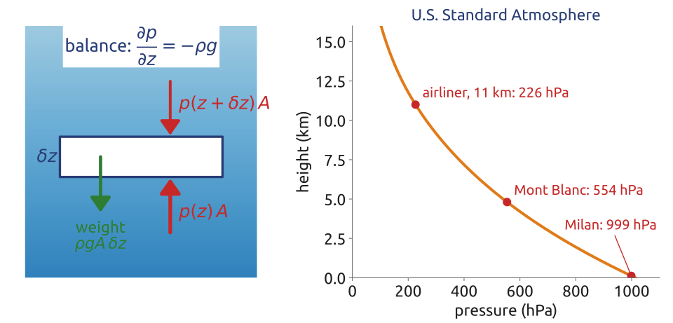
\[\begin{aligned} \frac{\partial p}{\partial z} = -\rho g \quad&\Longrightarrow\quad p(z) = \int_z^{\infty}\rho g\,dz'\\[8pt] \text{with } p = \rho R T: \quad&\phantom{\Longrightarrow}\quad \frac{1}{p}\frac{\partial p}{\partial z} = -\frac{g}{RT} = -\frac{1}{H_\rho} \end{aligned}\]

\(p(z)\): the weight of the fluid above, per unit area; \(R\): gas constant of air; \(T\): temperature; \(H_\rho = RT/g\): scale height, over which \(p\) falls by a factor \(e\)

Pressure is the weight of the fluid above: no vertical motion to forecast, no vertical sound waves

(Vallis 2017, sec. 1.3.3 and sec. 2.7; Holton 2004, sec. 1.6)

Slab: p(z) A up, p(z + dz) A down, weight rho g A dz. With p = rho R T at constant T: dp/p = -g dz/(RT): exponential. Torricelli and Pascal (lecture 1) measured exactly this.

A parcel lifted without heating

• Lift a small parcel of dry air, too fast to exchange heat with the air around it
• Its pressure is that of the air around it: it falls, the parcel expands, and expanding, it cools

\[\begin{aligned} &\text{first law:} && c_p\frac{DT}{Dt} - \frac{1}{\rho}\frac{Dp}{Dt} = Q\\[4pt] &\text{no heating, } Q = 0\text{:} && c_p\,dT = \frac{dp}{\rho} = -g\,dz\\[4pt] &\Longrightarrow && \Gamma_d \equiv -\frac{dT}{dz} = \frac{g}{c_p} = 9.8\ \text{K/km} \end{aligned}\]

\(Q\): heating rate (W/kg); \(dT\), \(dp\): changes following the parcel; \(dp = -\rho g\,dz\): hydrostatic balance of the air around it; \(c_p = 1004\) J/(kg K): specific heat of dry air at constant pressure

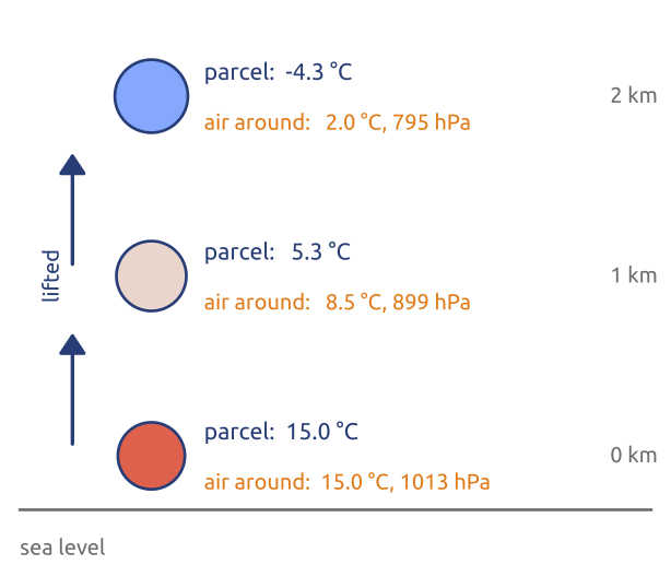
A dry parcel lifted without heating cools by about 10 K per km: the dry adiabatic lapse rate

(Holton 2004, sec. 2.7.2, eqs. 2.47–2.48; Vallis 2017, sec. 2.10.2)

Ask first: lift a parcel 1 km without heating: how much colder? (Most guess a degree or two.) Board: first law c_p dT - (1/rho) dp = 0; the parcel’s pressure is the environment’s, dp = -rho g dz (rho of the parcel and of the air nearly equal). Same for every dry parcel, at every height: it keeps its theta. The air around it cools at 6.5 K/km on average: next slide.

Static stability: vertical displacements of dry air

• Stable: a parcel pushed up or down comes back. Unstable: it keeps going (convection)
• At the same pressure, colder air is denser, since \(p = \rho R T\): a parcel colder than the air around it sinks, a warmer one rises
• Lifted, the parcel cools at \(\Gamma_d\); the air around it at its own lapse rate \(\Gamma = -\partial T/\partial z\)

\[\begin{aligned} \frac{T}{\theta}\frac{\partial\theta}{\partial z} &= \Gamma_d - \Gamma\\[4pt] \text{stable} \iff \Gamma < \Gamma_d &\iff \frac{\partial\theta}{\partial z} > 0 \end{aligned}\]

\(\theta\): potential temperature, kept by the parcel

• Mean atmosphere, 6.5 K/km: stable. Just above sun-heated ground \(\Gamma > \Gamma_d\): thermals

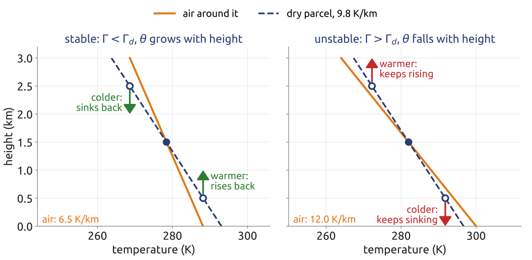
Stable when \(\theta\) grows with height: a displaced parcel is pushed back to its level

(Holton 2004, sec. 2.7.3, eq. 2.49; Vallis 2017, sec. 2.10.2)

Ask first: a parcel pushed down 1 km in the standard atmosphere: warmer or colder than the air around it? (Warmer: it warms at 9.8 K/km, the air at 6.5.) Holton 2.49 from the log of theta, hydrostatic and gas law. The parcel keeps theta: above it the air has higher theta, so it is heavier there. Moist air: latent heat, smaller lapse rate (about 6 K/km), conditional instability: not today. The restoring force gives oscillations, frequency N (lecture 4).

In class: how thick is the atmosphere?

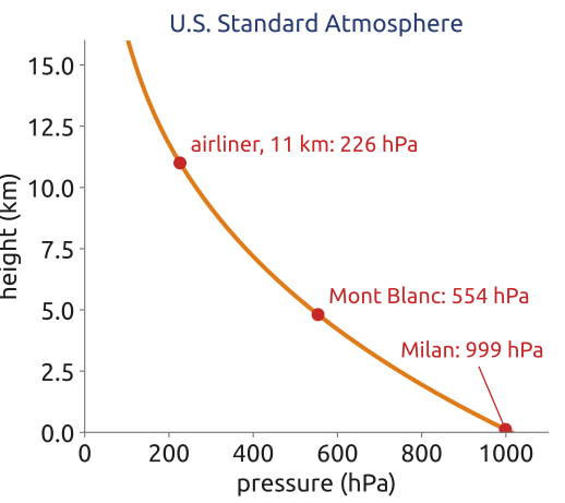
Exercise 1 — How thick is the atmosphere? (a) With hydrostatic balance and the gas law, show that an atmosphere at constant temperature \(T\) has \(p = p_0\,e^{-z/H_\rho}\) with the scale height \(H_\rho = RT/g\). Compute \(H_\rho\) for \(T = 250\) K, and the pressure at Mont Blanc (4808 m) and at 11 km as fractions of \(p_0\). (b) The föhn, a warm, dry wind down the lee side of the Alps (the side sheltered from the wind): dry air crosses them at 3000 m at \(-5\,{}^\circ\)C and comes down to Milan (120 m) without heating. How warm does it arrive? Would an atmosphere cooling by 12 K/km be stable?

\(R = 287\) J/(kg K), \(c_p = 1004\) J/(kg K), \(g = 9.81\) m/s². Potential temperature: \(\theta = T(p_0/p)^{R/c_p}\).

(c) Mars. The Martian atmosphere is carbon dioxide, \(R = 189\) J/(kg K), \(c_p = 770\) J/(kg K), with \(g = 3.71\) m/s\(^2\) and a typical temperature of 210 K. Compute its scale height and its dry adiabatic lapse rate. Its surface pressure is only about 6 hPa: is the Martian atmosphere thinner or thicker than the Earth’s, in kilometres?

In notebook 03a: open in Colab · download

(Holton 2004, secs. 1.6.1, 2.7.2–2.7.3; Vallis 2017, sec. 1.3.3)

1. H = 7.3 km; Mont Blanc 0.52 p0 (525 hPa), 11 km 0.22 p0. (b) -5 C + 9.8 K/km x 2.88 km = 23 C in Milan (the foehn: warm, dry wind; moist on the windward side, it cooled more slowly there). 12 K/km > Gamma_d: unstable.
2. Mars: H = 10.7 km, Gamma_d = 4.8 K/km: thicker in km (low g), thinner in mass.

What the exercise showed

• Isothermal: \(p = p_0\,e^{-z/H_\rho}\), \(H_\rho = RT/g = 7.3\) km at 250 K: half the air lies below Mont Blanc, three quarters below 11 km
• The pressure at a height depends on the mean of \(1/T\) below it: a warm column is thick
• Föhn: dry air coming down 2.9 km warms by 28 K, from \(-5\) to \(23\,^\circ\)C; 12 K/km would be unstable
• Mars: \(H_\rho = 10.7\) km, thicker in km; 60 times less air

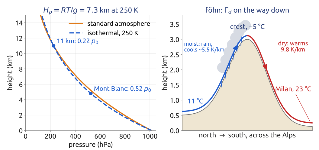
The air thins by \(e\) every 7 km or so, and cools with height more slowly than \(\Gamma_d\): it is stable

(Holton 2004, secs. 1.6.1, 2.7.2–2.7.3; Vallis 2017, sec. 1.3.3) · Standard atmosphere: U.S. Standard Atmosphere (1976)

Two minutes, after the exercise. Answers: H = 7.3 km; Mont Blanc 0.52 p0, 11 km 0.22 p0 (the standard atmosphere 0.55 and 0.22: the mean of 1/T up to 11 km is 1/(251 K)); Gamma_d = 9.8 K/km; Mars 10.7 km, 4.8 K/km, 162 kg/m2 of air against 10 300. Warm columns thick: thermal wind (notebook 03a, exercise 1.2).

The ocean (1/2): density hardly changes

Seawater: \(\rho\) grows by 2 % over 4 km, mostly by compression; 20 K of warming changes it by 0.3 %, 5 g/kg of salt by 0.4 %

\[\begin{aligned} &\text{momentum:} && \rho\Big(\frac{D\mathbf{u}}{Dt} + 2\boldsymbol{\Omega}\times\mathbf{u}\Big) = -\nabla p - \rho g\,\mathbf{k}\\[4pt] &\text{write:} && {\color{#1f5ccc}{\rho = \rho_0 + \delta\rho,\quad |\delta\rho| \ll \rho_0}}\\[2pt] & && {\color{#1f5ccc}{p = \tilde p(z) + \delta p,\quad \frac{d\tilde p}{dz} = -\rho_0 g}}\\[4pt] &\Longrightarrow && (\rho_0 + \delta\rho)\Big(\frac{D\mathbf{u}}{Dt} + 2\boldsymbol{\Omega}\times\mathbf{u}\Big) = -\nabla\delta p - g\,\delta\rho\,\mathbf{k} \end{aligned}\]

\(\rho_0 = 1027\) kg/m³: a constant reference density; \(\tilde p(z)\): the hydrostatic pressure of \(\rho_0\) alone; \(\delta\rho\), \(\delta p\): the departures from them

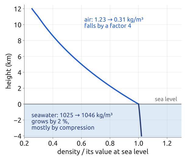
The weight of \(\rho_0\) is held up by \(\tilde p(z)\): only the density anomaly \(\delta\rho\) is left to push the water

(Vallis 2017, secs. 2.4.1–2.4.2, eqs. 2.88–2.93; Cushman-Roisin and Beckers 2011, sec. 3.7)

Ask first: seawater density varies by a few tenths of a percent: why not treat it as constant everywhere? (Then nothing would sink or float: no thermohaline circulation.) Numbers with beta_T = 1.7e-4 1/K, beta_S = 7.6e-4 per g/kg (lecture 2). Board: split rho and p, use d(p~)/dz = -rho0 g: nothing dropped yet.

The ocean (2/2): the Boussinesq equations

• Divide by \(\rho_0\) and drop \(\delta\rho/\rho_0 \sim 10^{-3}\) next to the acceleration, but not next to \(g\): \(\delta\rho\) is small, but \(g\) is big
• Mass, \(D\delta\rho/Dt + (\rho_0 + \delta\rho)\nabla\cdot\mathbf{u} = 0\): the first term is \(10^{-3}\) of the second

\[\begin{aligned} \frac{D\mathbf{u}}{Dt} + 2\boldsymbol{\Omega}\times\mathbf{u} &= -\frac{1}{\rho_0}\nabla\delta p + {\color{#1f5ccc}{b\,\mathbf{k}}}\\ \nabla\cdot\mathbf{u} &= 0, \qquad \frac{Db}{Dt} = \dot b\\ b = -g\,\frac{\delta\rho}{\rho_0} &= g\,\big[\beta_T(T - T_0) - \beta_S(S - S_0)\big] \end{aligned}\]

\(b\): buoyancy; \(\dot b\): its sources, by heating and salt fluxes; \(T\), \(S\): temperature, salinity; \(T_0\), \(S_0\): reference values; \(\beta_T\), \(\beta_S\): thermal expansion and haline contraction coefficients

• Volume is conserved: no sound waves. Density changes only by heat and salt

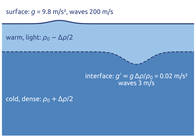
Across a density jump \(\Delta\rho\), a displaced interface feels only the reduced gravity \(g' = g\,\Delta\rho/\rho_0\)

Density matters only through buoyancy: inside the ocean, gravity is a weak \(g' \ll g\)

(Vallis 2017, sec. 2.4.2, eqs. 2.94–2.101; Cushman-Roisin and Beckers 2011, sec. 3.7)

Boussinesq (1903). Vallis writes phi = delta p/rho0. Not “D(delta rho)/Dt = 0”: density changes come from the thermodynamic equation and the equation of state. Reduced gravity: the thermocline feels g’ = 0.02 m/s^2, waves at 3 m/s (the notebook’s beta-plane eddy uses it); hence the small ocean deformation radius. Air is not Boussinesq over its whole depth (density falls by 3 in 10 km): anelastic or pressure coordinates; fine for shallow layers.

Primitive equations (1/2): on the sphere

\[\begin{aligned} \frac{Du}{Dt} - 2\Omega v\sin\varphi + {\color{#c62828}{2\Omega w\cos\varphi}} - \frac{uv\tan\varphi}{{\color{#1f5ccc}{r}}} + {\color{#c62828}{\frac{uw}{r}}} &= -\frac{1}{\rho\,{\color{#1f5ccc}{r}}\cos\varphi}\frac{\partial p}{\partial\lambda}\\ \frac{Dv}{Dt} + 2\Omega u\sin\varphi + \frac{u^2\tan\varphi}{{\color{#1f5ccc}{r}}} + {\color{#c62828}{\frac{vw}{r}}} &= -\frac{1}{\rho\,{\color{#1f5ccc}{r}}}\frac{\partial p}{\partial\varphi}\\ {\color{#2e7d32}{\frac{Dw}{Dt} - 2\Omega u\cos\varphi - \frac{u^2 + v^2}{r}}} &= -\frac{1}{\rho}\frac{\partial p}{\partial r} - g \end{aligned}\]

\(\lambda\): longitude; \(\varphi\): latitude; \(r\): distance from the centre of the Earth; \(u\), \(v\), \(w\): eastward, northward, upward velocity; \(D/Dt = \partial/\partial t + (u/{\color{#1f5ccc}{r}}\cos\varphi)\,\partial/\partial\lambda + (v/{\color{#1f5ccc}{r}})\,\partial/\partial\varphi + w\,\partial/\partial r\)

• The axes turn as the parcel moves over the sphere: metric terms in \(1/r\). For thin, large-scale flow:
• Hydrostatic: the green terms, \(10^{-3}\) m/s² or less, against 10 m/s² for the pressure force and gravity
• Shallow fluid: \(r = a + z\), with \(z\) below 100 km against \(a = 6371\) km, is very nearly \(a\)
• Traditional: the red terms, Coriolis and metric terms with \(w\), are tiny since \(w \sim 1\) cm/s \(\ll u\)

Three approximations for thin, large-scale flow: hydrostatic, shallow fluid, traditional

(Vallis 2017, sec. 2.2.3, eq. 2.47)

Vallis 2.47 expanded. Colours match the next slide: green dropped by hydrostatic balance, blue r replaced by a, red dropped by the traditional approximation.

Primitive equations (2/2): what is left

\[\begin{aligned} \frac{Du}{Dt} - f v - \frac{uv\tan\varphi}{a} &= -\frac{1}{\rho\,a\cos\varphi}\frac{\partial p}{\partial\lambda}\\ \frac{Dv}{Dt} + f u + \frac{u^2\tan\varphi}{a} &= -\frac{1}{\rho\,a}\frac{\partial p}{\partial\varphi}\\ 0 &= -\frac{1}{\rho}\frac{\partial p}{\partial z} - g \end{aligned}\]

\(f = 2\Omega\sin\varphi\); with mass, the gas law and the first law

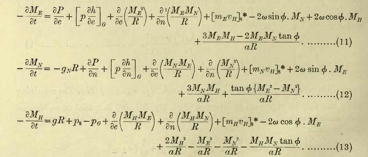
Richardson (1922), p. 34: the same equations in flux form; every term kept, but \(a\) for \(r\). Public domain

• Hydrostatic: \(w\) diagnosed; no vertical sound waves, only the horizontal Lamb wave
• Shallow fluid and traditional only together: energy, angular momentum kept
• Ocean, Boussinesq (\(\rho \to \rho_0\) except in \(b\), \(\nabla\cdot\mathbf{u} = 0\)): no sound waves; used by almost all ocean models
• Used by most climate models, and by most weather models until about a decade ago (now non-hydrostatic, compressible)

\[\begin{aligned} \frac{\partial w}{\partial z} &= -\nabla_h\cdot\mathbf{u}_h\\ \Longrightarrow\quad w(z) &= -\int_{-H}^{z}\nabla_h\cdot\mathbf{u}_h\,dz' \end{aligned}\]

\(\mathbf{u}_h\), \(\nabla_h\): horizontal; ocean bottom at \(-H\); air: the same in \(p\), \(\omega = Dp/Dt\)

Atmosphere: no vertical sound waves. Ocean: no sound waves at all

(Vallis 2017, sec. 2.2.4, eqs. 2.48–2.50; Phillips 1966; White et al. 2005; Richardson 1922, Ch. 4/4) · Equations: archive.org: Weather prediction by numerical process

Phillips (1966): drop the cos terms and the uw/r, vw/r terms together, or energy and angular momentum are not conserved. White et al. (2005): the consistent family of approximations.

The f-plane and the beta-plane

Near a latitude \(\varphi_0\), use flat coordinates \(x\) (east), \(y\) (north), and expand \(f\):

\[f \approx f_0 + {\color{#1f5ccc}{\beta y}}, \qquad \beta = \frac{2\Omega\cos\varphi_0}{a}\]

• f-plane: \(f = f_0\); at Milan \(1.04\times10^{-4}\ \mathrm{s^{-1}}\)
• beta-plane: \(\beta = 1.6\times10^{-11}\ \mathrm{m^{-1}s^{-1}}\) at \(45^\circ\): \(f\) grows by 15 % in 1000 km
• Small, but it makes the Rossby waves and the western boundary currents

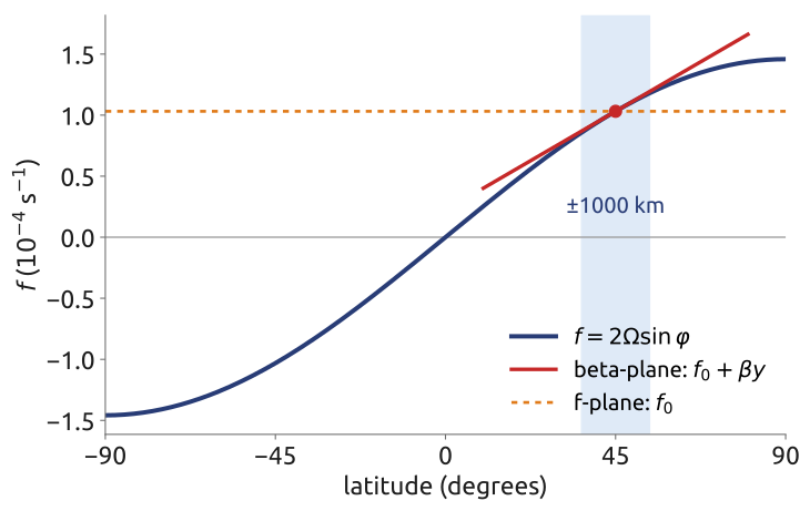
Flat geometry, with the curvature of the Earth kept only in the variation of \(f\)

(Vallis 2017, sec. 2.3; Cushman-Roisin and Beckers 2011, sec. 9.4)

Rossby (1939) introduced the beta-plane. Valid for scales well below the radius of the Earth. Equatorial beta-plane: f = beta y.

Primitive equations on the beta-plane

\[\begin{aligned} \frac{Du}{Dt} - f v\;{\color{#6e6e6e}{-\;\frac{uv\tan\varphi}{a}}} &= -\frac{1}{\rho}\frac{\partial p}{\partial x}\\ \frac{Dv}{Dt} + f u\;{\color{#6e6e6e}{+\;\frac{u^2\tan\varphi}{a}}} &= -\frac{1}{\rho}\frac{\partial p}{\partial y}\\ \frac{\partial p}{\partial z} &= -\rho g, \qquad f = f_0 + \beta y \end{aligned}\]

\(f_0 = 2\Omega\sin\varphi_0\); \(\beta = 2\Omega\cos\varphi_0/a\); \(x = a\lambda\cos\varphi_0\), \(y = a(\varphi - \varphi_0)\): eastward and northward distances on the plane tangent at \(\varphi_0\); \(D/Dt = \partial/\partial t + u\,\partial/\partial x + v\,\partial/\partial y + w\,\partial/\partial z\). Grey: metric terms, of size \(U^2/a\), \(L/a\) times the acceleration: dropped

• Atmosphere: with mass, \(D\rho/Dt + \rho\nabla\cdot\mathbf{u} = 0\), the gas law and the first law
• Ocean, Boussinesq: \(\rho \to \rho_0\) and \(p \to \delta p\) on the right, \(\partial\delta p/\partial z = \rho_0 b\), \(\nabla\cdot\mathbf{u} = 0\), \(Db/Dt = \dot b\)
• f-plane, \(f = f_0\): the form used from here on for shallow water, the Ekman layer, quasi-geostrophy

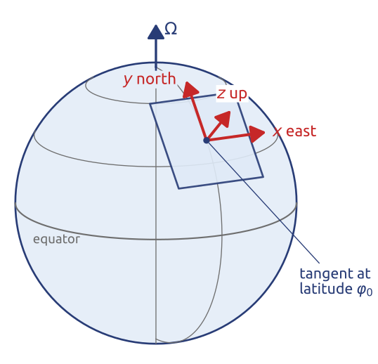
On a plane tangent to the Earth: Cartesian equations, with the sphere left only in \(f = f_0 + \beta y\)

(Vallis 2017, sec. 2.3, eqs. 2.78, 2.81–2.83; Cushman-Roisin and Beckers 2011, sec. 9.4)

Valid for L much smaller than a: the metric terms are L/a times the acceleration. Vallis keeps only f = f0 + beta y: “sphericity combined with rotation is dynamically equivalent to a differentially rotating system”. The beta term is kept although beta L/f0 is also small, because it changes the vorticity dynamics (Rossby waves).

Shallow water (1/6): one layer

• One layer of fluid of constant density \(\rho_0\), thin: depth \(\ll\) width
• Free surface at \(z = \eta\), bottom at height \(\eta_b\) above \(z = -H\)
• Depth: \(h = H + \eta - \eta_b\)
• Unknowns: \(\mathbf{u} = (u, v)\) and \(h\) (or \(\eta\)), functions of \(x, y, t\) only

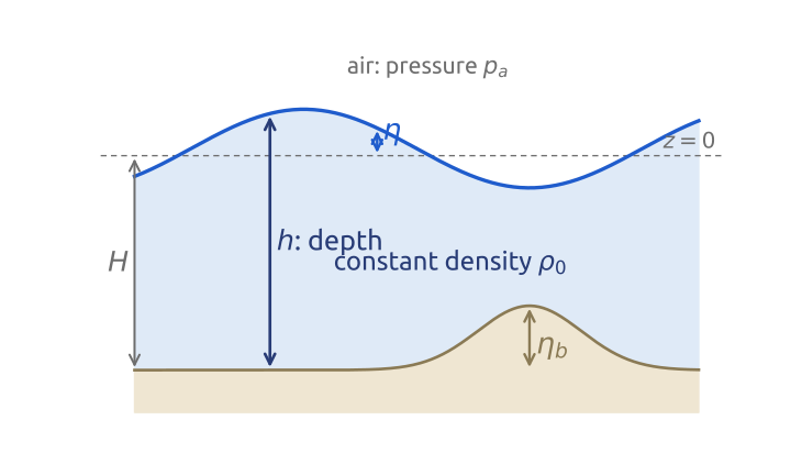
The simplest fluid with rotation, gravity waves and balance: Laplace’s ocean (1776)

(Vallis 2017, sec. 3.1; Cushman-Roisin and Beckers 2011, sec. 7.3)

Laplace: lecture 1. A model of the ocean (above the thermocline) or of the atmosphere’s first mode. Vertical scale exaggerated in the figure.

Shallow water (2/6): hydrostatic pressure

Integrate hydrostatic balance from a height \(z\) up to the surface, where \(p = p_a\):

\[\begin{aligned} \int_z^{\eta}\frac{\partial p}{\partial z'}\,dz' &= -\int_z^{\eta}\rho_0 g\,dz'\\ \Longrightarrow\quad p(x, y, z, t) &= p_a + \rho_0 g\,\big(\eta(x, y, t) - z\big)\\ \Longrightarrow\quad -\frac{1}{\rho_0}\nabla p &= {\color{#1f5ccc}{-g\,\nabla\eta}} \end{aligned}\]

\(p_a\): pressure of the air above, uniform; \(\nabla = (\partial_x, \partial_y)\)

The same horizontal force at every depth.

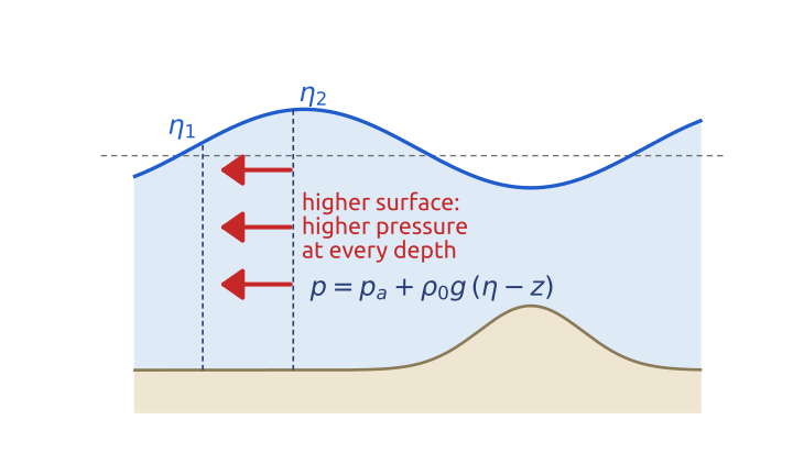
Higher surface, higher pressure at every depth: the surface slope pushes the whole column

(Vallis 2017, sec. 3.1.1, eqs. 3.1–3.4; Cushman-Roisin and Beckers 2011, sec. 7.3)

The pressure gradient does not depend on z because the density is constant. Vallis takes p = 0 at the surface.

Shallow water (3/6): columns move as columns

\[\begin{aligned} &\text{primitive equations, } \rho = \rho_0: && \frac{\partial\mathbf{u}}{\partial t} + (\mathbf{u}\cdot\nabla)\mathbf{u} + {\color{#c62828}{w\,\frac{\partial\mathbf{u}}{\partial z}}} + f\,\mathbf{k}\times\mathbf{u} = {\color{#1f5ccc}{-\frac{1}{\rho_0}\nabla p}}\\[2pt] &\text{hydrostatic pressure:} && {\color{#1f5ccc}{-\frac{1}{\rho_0}\nabla p = -g\nabla\eta}}\text{, the same at every } z \;\Longrightarrow\; \mathbf{u} = \mathbf{u}(x, y, t),\; {\color{#c62828}{w\,\frac{\partial\mathbf{u}}{\partial z} = 0}}\\[2pt] &\Longrightarrow && \underbrace{\frac{\partial\mathbf{u}}{\partial t}}_{\text{local change}} + \underbrace{(\mathbf{u}\cdot\nabla)\mathbf{u}}_{\text{nonlinear advection}} = \underbrace{-f\,\mathbf{k}\times\mathbf{u}}_{\text{Coriolis}}\;\underbrace{-\,g\nabla(h + \eta_b)}_{\text{pressure}} \end{aligned}\]

\(\mathbf{u} = (u, v)\), \(\nabla = (\partial_x, \partial_y)\); \(\eta = h + \eta_b - H\); \(f\,\mathbf{k}\times\mathbf{u} = (-fv, fu)\)

• Same push at every depth: \(-g\nabla\eta\) has no \(z\) in it (constant \(\rho_0\), hydrostatic)
• \(w\) is still there (it lifts the surface: next slide), but \(\partial\mathbf{u}/\partial z = 0\) kills \(w\,\partial\mathbf{u}/\partial z\)

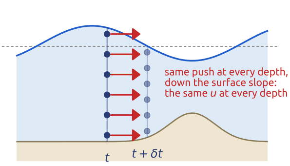
Vertical columns of fluid stay vertical and move as a whole

(Vallis 2017, sec. 3.1.1, eqs. 3.6–3.8; Cushman-Roisin and Beckers 2011, sec. 7.3)

Not Taylor–Proudman: the z-independence of u comes from hydrostatic balance with constant density (Vallis 3.1.1), with or without rotation. Friction and wind stress would add terms. f: constant (f-plane) or f0 + beta y.

Shallow water (4/6): mass, from the 3D equation

3D, constant \(\rho_0\), with \(\mathbf{v} = (u, v, w)\) the 3D velocity and \(\nabla_3\) the 3D gradient: \(\nabla_3\cdot\mathbf{v} = 0\), so \(\dfrac{\partial w}{\partial z} = -\nabla\cdot\mathbf{u}\), with \(\mathbf{u} = (u, v)\) horizontal only. Integrate from the bottom, \(z_b = -H + \eta_b\), to the surface (\(\nabla\cdot\mathbf{u}\) has no \(z\)):

\[\int_{z_b}^{\eta}\frac{\partial w}{\partial z}\,dz = -\int_{z_b}^{\eta}\nabla\cdot\mathbf{u}\,dz \;\Longrightarrow\; w\big|_{\eta} - w\big|_{z_b} = -h\,\nabla\cdot\mathbf{u}\]

A particle on the surface stays on it; the bottom does not move:

\[w\big|_{\eta} = \frac{D\eta}{Dt}, \qquad w\big|_{z_b} = \frac{Dz_b}{Dt} = \mathbf{u}\cdot\nabla\eta_b \;\Longrightarrow\; \frac{D(\eta - z_b)}{Dt} = -h\,\nabla\cdot\mathbf{u}\]

Kinematic condition: \(D/Dt\), not \(\partial/\partial t\), because the particle also slides along the surface: its height \(\eta(x_p(t), y_p(t), t)\) changes by \(\partial\eta/\partial t + \mathbf{u}\cdot\nabla\eta\). Over the bump \(\partial\eta_b/\partial t = 0\), yet the flow climbs it: \(w = \mathbf{u}\cdot\nabla\eta_b\).

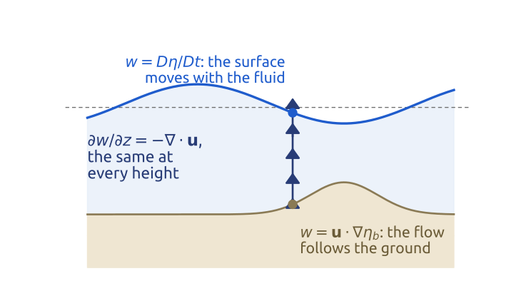
\[\frac{Dh}{Dt} = -h\,\nabla\cdot\mathbf{u} \;\Longleftrightarrow\; \frac{\partial h}{\partial t} + \nabla\cdot(h\mathbf{u}) = 0\]

\(h = \eta - z_b = \eta + H - \eta_b\); \(\nabla = (\partial_x, \partial_y)\); \(D/Dt = \partial/\partial t + \mathbf{u}\cdot\nabla\)

Converging columns get taller: the surface rises

(Vallis 2017, sec. 3.1.2, eqs. 3.15–3.19; Cushman-Roisin and Beckers 2011, sec. 7.3)

The kinematic conditions: the free surface is made of the same particles at all times, so its height changes as they move up, w = D eta/Dt. Integrate the 3D incompressibility over the depth.

Shallow water (5/6): the equations

\[\begin{aligned} \frac{\partial\mathbf{u}}{\partial t} + (\mathbf{u}\cdot\nabla)\mathbf{u} + f\,\mathbf{k}\times\mathbf{u} &= -g\nabla(h + \eta_b)\\ \frac{\partial h}{\partial t} + \underbrace{\mathbf{u}\cdot\nabla h}_{\text{transport}} &= \underbrace{-h\,\nabla\cdot\mathbf{u}}_{\text{flow divergence}}\\ \text{or, in flux form:}\quad \frac{\partial h}{\partial t} + \nabla\cdot(h\mathbf{u}) &= 0 \end{aligned}\]

Linearized about rest (small \(\eta\) and \(\mathbf{u}\): drop \((\mathbf{u}\cdot\nabla)\mathbf{u}\), \(h\mathbf{u} \to H\mathbf{u}\)), flat bottom: Laplace’s tidal equations (1776)

\[\frac{\partial\mathbf{u}}{\partial t} + f\,\mathbf{k}\times\mathbf{u} = -g\nabla\eta, \qquad \frac{\partial\eta}{\partial t} + H\,\nabla\cdot\mathbf{u} = 0\]

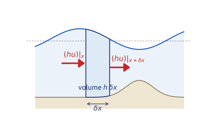
Flux form: what flows in through the sides of a column, minus what flows out, raises it.

Three equations, three unknowns \(u, v, h\): the standard test bed of weather and ocean numerics

(Vallis 2017, sec. 3.1; Hendershott 1981)

Flux form = the box of the continuity derivation, now a column: finite volumes start from it. Linear version: drop (u . grad)u and replace h by H in the flux. On the sphere: the same with metric terms.

Shallow water (6/6): the vector-invariant form

Rewrite the advection with a vector identity, with \(\zeta = \partial_x v - \partial_y u\) the relative vorticity and \(K = |\mathbf{u}|^2/2\) the kinetic energy:

\[(\mathbf{u}\cdot\nabla)\mathbf{u} = \zeta\,\mathbf{k}\times\mathbf{u} + \nabla K\]

Put it in the momentum equation; gather \(\zeta + f\) in front of \(\mathbf{k}\times\mathbf{u}\) and the gradients in \(B\):

\[\frac{\partial\mathbf{u}}{\partial t} + (\zeta + f)\,\mathbf{k}\times\mathbf{u} = -\nabla B\]

Write \((\zeta + f)\,\mathbf{u} = Q\,h\mathbf{u}\):

\[\frac{\partial\mathbf{u}}{\partial t} + Q\,\mathbf{k}\times(h\mathbf{u}) = -\nabla B, \qquad \frac{\partial h}{\partial t} + \nabla\cdot(h\mathbf{u}) = 0\]

\[B = \underbrace{\tfrac{1}{2}|\mathbf{u}|^2}_{K} + g\,(h + \eta_b)\]

kinetic plus potential energy, per unit mass

\[Q = \frac{\zeta + f}{h}\]

the spin of a column, \(\zeta + f\), per unit depth

• No coordinates in it: the same on the plane and on the sphere
• The form of C-grid models (MPAS, ICON): the mass flux \(h\mathbf{u}\) is shared by both equations

Vorticity and potential vorticity are already inside the momentum equation

(Vallis 2017, sec. 2.2.6 and sec. 3.7.1, eq. 3.94)

Exercise for the notebook: check the identity in components. Vallis 3.94 writes B = g eta + u^2/2, with his eta the surface height above the mean bottom (= h + eta_b here): the same B. The curl of this form gives the vorticity equation, next. TRiSK (Thuburn, Ringler, Skamarock, Klemp) discretizes exactly Q k x (hu).

Geostrophic balance in shallow water

\[\begin{array}{ccccc} {\color{#c62828}{\dfrac{\partial\mathbf{u}}{\partial t} + (\mathbf{u}\cdot\nabla)\mathbf{u}}} & + & f\,\mathbf{k}\times\mathbf{u} & = & -g\nabla\eta\\[6pt] {\color{#c62828}{U^2/L}} & & fU & & g\,\delta\eta/L\\[4pt] {\color{#c62828}{Ro}} & & 1 & & g\,\delta\eta/(fUL) \end{array}\]

\(U\), \(L\): speed and size; \(\delta\eta\): change of surface height over \(L\); time \(L/U\). Last row: over \(fU\)

For \(Ro = U/(fL) \ll 1\) the red acceleration drops. Pressure is then the only term left to balance Coriolis, so it must be of order 1 too: \(\delta\eta \sim fUL/g\)

\[f\,\mathbf{k}\times\mathbf{u}_g = -g\nabla\eta \;\Longleftrightarrow\; \mathbf{u}_g = \frac{g}{f}\,\mathbf{k}\times\nabla\eta\]

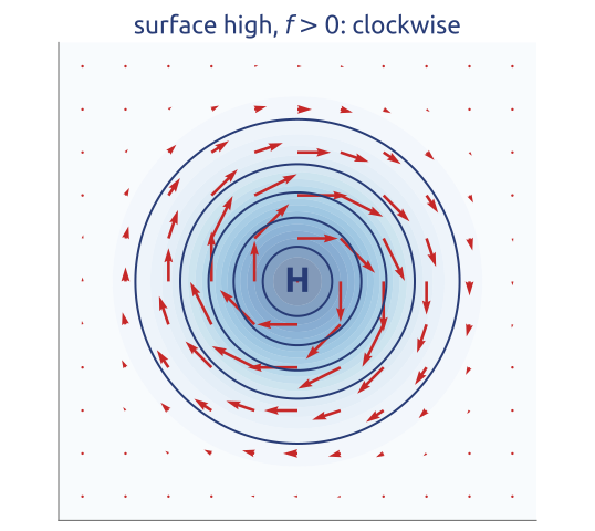
• Along the contours of \(\eta\): clockwise around a high (northern hemisphere)
• Gulf Stream, \(U = 1\) m/s, \(L = 100\) km: \(Ro = 0.1\), \(\delta\eta \approx 1\) m
• But: on the f-plane \(\nabla\cdot\mathbf{u}_g = 0\): \(\eta\) never changes

Geostrophy is a diagnostic relation: to predict, we need vorticity

(Vallis 2017, secs. 2.8.1–2.8.2 and sec. 3.5; Cushman-Roisin and Beckers 2011, secs. 4.5, 7.1)

Ferrel’s wind (lecture 1) for the shallow layer: surface slope instead of isobars. The degeneracy: geostrophic + continuity give d eta/dt = 0; the evolution is in the small ageostrophic part. g delta eta/(fUL) ~ 1 is not assumed: it follows, since nothing else can balance Coriolis (if the surface were flatter, Coriolis alone would turn u: inertial oscillations). Gulf Stream: about 1 m across it, seen by altimetry. Next: vorticity removes the pressure.

Vorticity (1/3): stretching spins up

Start from the vector-invariant momentum equation, \(\dfrac{\partial\mathbf{u}}{\partial t} + (\zeta + f)\,\mathbf{k}\times\mathbf{u} = -\nabla B\), and take its curl, \(\mathbf{k}\cdot\nabla\times\):

• \(\mathbf{k}\cdot\nabla\times\dfrac{\partial\mathbf{u}}{\partial t} = \dfrac{\partial\zeta}{\partial t} = \dfrac{\partial(\zeta + f)}{\partial t}\), since \(f\) does not depend on \(t\)
• \(\mathbf{k}\cdot\nabla\times\big[(\zeta + f)\,\mathbf{k}\times\mathbf{u}\big] = \nabla\cdot\big[(\zeta + f)\,\mathbf{u}\big]\)
• \(\mathbf{k}\cdot\nabla\times\nabla B = 0\): the pressure and the kinetic energy drop out

\[\frac{\partial(\zeta + f)}{\partial t} + \nabla\cdot\big[(\zeta + f)\,\mathbf{u}\big] = 0\]

\[\frac{D(\zeta + f)}{Dt} = {\color{#1f5ccc}{-(\zeta + f)\,\nabla\cdot\mathbf{u}}}\]

Expanding the divergence, \(\nabla\cdot[(\zeta + f)\mathbf{u}] = \mathbf{u}\cdot\nabla(\zeta + f) + (\zeta + f)\nabla\cdot\mathbf{u}\); \(\zeta + f\): absolute vorticity; \(Df/Dt = \beta v\). Converging, \(\nabla\cdot\mathbf{u} < 0\): the column spins faster

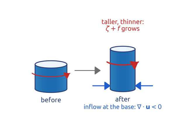
Like a skater pulling the arms in: squeezed sideways, a column spins faster

(Vallis 2017, sec. 3.7.1, eqs. 3.93–3.95; Cushman-Roisin and Beckers 2011, sec. 7.4)

Identity: k . curl(a k x u) = div(a u) for horizontal u and any scalar a (write it in components: k x u = (-v, u)). The vorticity equation in flux form is a conservation law for zeta + f, like mass for h. Kelvin’s circulation for a thin column (lecture 1).

Vorticity (2/3): potential vorticity

Two equations with the same divergence:

\[\frac{D(\zeta + f)}{Dt} = -(\zeta + f)\,\nabla\cdot\mathbf{u}, \qquad \frac{Dh}{Dt} = -h\,\nabla\cdot\mathbf{u}\]

Eliminate \(\nabla\cdot\mathbf{u}\): for \(Q = (\zeta + f)/h\), by the quotient rule,

\[\frac{DQ}{Dt} = \frac{1}{h}\frac{D(\zeta + f)}{Dt} - \frac{\zeta + f}{h^2}\frac{Dh}{Dt} = -\frac{\zeta + f}{h}\,\nabla\cdot\mathbf{u} + \frac{\zeta + f}{h}\,\nabla\cdot\mathbf{u} = 0\]

\[\frac{D}{Dt}\left(\frac{\zeta + f}{h}\right) = 0\]

• Each column keeps its own \(Q\): one scalar carried by the flow holds the dynamics
• Rossby (1936, 1940); Ertel (1942) for any stratified fluid

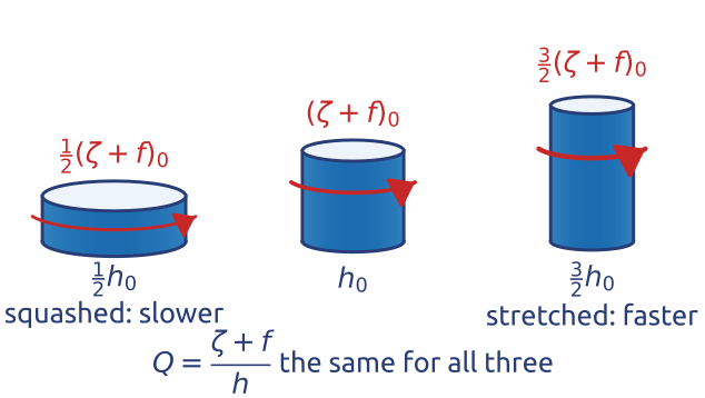
Taller columns spin faster, shorter ones slower, in proportion

(Rossby 1940; Vallis 2017, sec. 3.7.1)

Equivalently: D(zeta+f)/Dt / (zeta+f) = -div u = Dh/Dt / h, so D ln((zeta+f)/h)/Dt = 0. Rossby 1940 named it “potential vorticity”. Without forcing and friction.

Vorticity (3/3): a column crossing a ridge

A column of ocean at \(45^\circ\)N, 4000 m tall, at rest (\(\zeta = 0\)), drifts east over a ridge on the sea floor (an underwater mountain range), where the ocean is 3000 m deep:

\[\frac{\zeta + f}{3000\ \mathrm{m}} = \frac{f_0}{4000\ \mathrm{m}} \quad\Rightarrow\quad \zeta + f = \tfrac{3}{4}f_0\]

\(f_0 = f(45^\circ\mathrm{N}) = 2\Omega\sin 45^\circ = 1.03\times10^{-4}\,\mathrm{s^{-1}}\), \(\Omega = 7.29\times10^{-5}\,\mathrm{s^{-1}}\)

• (a) It stays at \(45^\circ\)N: \(\zeta = -\tfrac{1}{4}f_0 = -2.6\times10^{-5}\,\mathrm{s^{-1}}\), it turns clockwise
• (b) It does not spin: \(\sin\varphi = \tfrac{3}{4}\sin 45^\circ\), it follows a contour of \(f/h\) down to \(32^\circ\)N, towards the equator

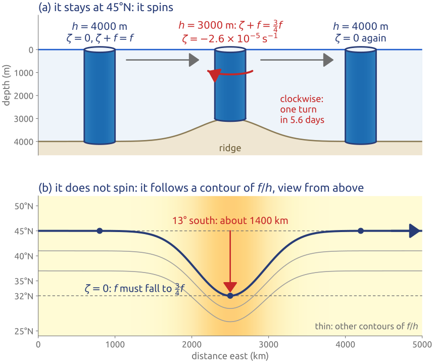
In general some of both: potential vorticity steers the flow, depth and latitude act alike

(Holton 2004, sec. 4.3; Vallis 2017, sec. 3.7.1)

Ask first: over the ridge, which way does it turn? Solid body: zeta = twice the angular velocity, so one turn takes 4 pi/|zeta| = 5.6 days. f/h contours: “geostrophic contours”. Real oceans: the Mid-Atlantic Ridge rises 2-3 km above a 4-5 km deep floor. Same mechanism as the Rossby waves (beta); an analogy with Taylor columns.

Example: eastward winds over the Rockies

An eastward wind, \(U = 15\) m/s, carries a column of air at \(45^\circ\mathrm{N}\), from the ground to the tropopause, 10 km tall, with \(\zeta = 0\), over a range 2500 m high. It keeps \((\zeta + f)/h\):

• Over the crest, squeezed to 7.5 km (already a little south): \(\zeta + f = \tfrac{3}{4}f_0\), \(\zeta \approx -2.5\times10^{-5}\,\mathrm{s^{-1}}\), anticyclonic: it turns towards the equator
• Past the range, 10 km tall again but at \(38^\circ\)N: \(\zeta = f_0 - f = +1.3\times10^{-5}\,\mathrm{s^{-1}}\), cyclonic: a lee trough (a low-pressure system), 1300 km east of the crest
• Then a ridge (high pressure) at \(52^\circ\)N, and so on: a train of troughs and ridges that stands still

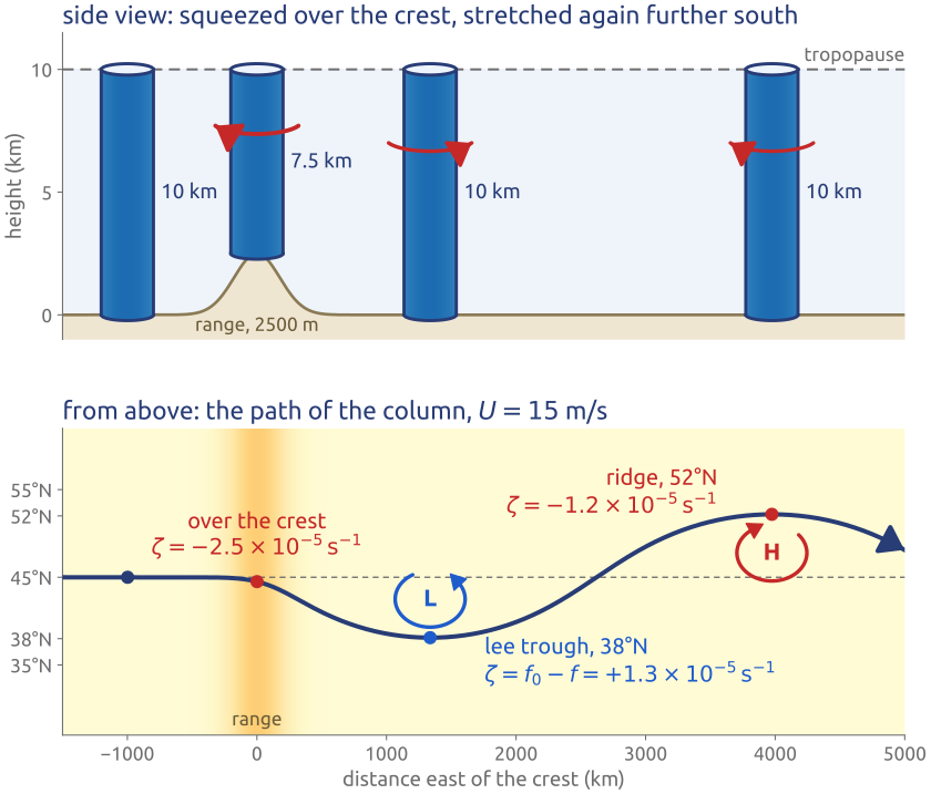
Squeezed over the mountains, stretched again further south: a trough in the lee of the Rockies

(Holton 2004, sec. 4.3, Fig. 4.9)

Ask first: past the mountains the column is 10 km tall again: is zeta back to zero? (No: it is further south, f is smaller.) The path is computed: zeta = U times its curvature, i.e. the heading turns at the rate zeta/U, zeta from the PV; no upstream stretching. Wavelength about 5300 km here (linear: 2 pi sqrt(U/beta) = 6000 km). Westward winds over the same range give no wave downstream (Holton Fig. 4.10). Real: the trough east of the Rockies, where lee cyclones form.

Linear waves (1/2): an eigenvalue problem

Laplace’s tidal equations (f-plane, flat bottom, depth \(H\)) and a plane wave:

\[(u, v, \eta) = (\hat u, \hat v, \hat\eta)\,e^{i(kx + ly - \omega t)}: \qquad \partial_t \to -i\omega,\quad \partial_x \to ik,\quad \partial_y \to il\]

\[\begin{alignedat}{11} &\frac{\partial u}{\partial t} && && {}- f v && {}+ g\frac{\partial\eta}{\partial x} && {}= 0 &&\quad\Longrightarrow\quad && {-i\omega\,\hat u} && && {}- f\,\hat v && {}+ igk\,\hat\eta && {}= 0\\[4pt] &\frac{\partial v}{\partial t} && {}+ f u && && {}+ g\frac{\partial\eta}{\partial y} && {}= 0 &&\quad\Longrightarrow\quad && {-i\omega\,\hat v} && {}+ f\,\hat u && && {}+ igl\,\hat\eta && {}= 0\\[4pt] &\frac{\partial\eta}{\partial t} && {}+ H\frac{\partial u}{\partial x} && {}+ H\frac{\partial v}{\partial y} && && {}= 0 &&\quad\Longrightarrow\quad && {-i\omega\,\hat\eta} && {}+ iHk\,\hat u && {}+ iHl\,\hat v && && {}= 0 \end{alignedat}\]

Three homogeneous linear equations for \(\hat u, \hat v, \hat\eta\): if their determinant is not zero, the only solution is \(\hat u = \hat v = \hat\eta = 0\); a wave needs a zero determinant:

\[i\omega\,\big(\omega^2 - f^2 - gH(k^2 + l^2)\big) = 0\]

\(\mathbf{K} = (k, l)\): wavevector, \(K^2 = k^2 + l^2\); \(\omega\): frequency; \(\hat u, \hat v, \hat\eta\): amplitudes

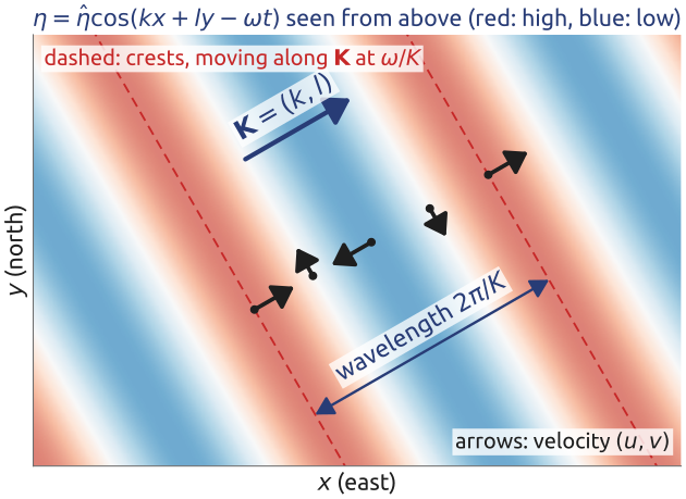
Three roots: one steady (geostrophic) mode and two waves travelling in opposite directions

(Vallis 2017, sec. 3.8; Cushman-Roisin and Beckers 2011, sec. 9.1)

Matrix form on the board if needed. Mathematicians: the eigenvalues of a skew-adjoint operator (with the energy inner product): real frequencies, no growth. Figure: a Poincare wave (K L_d = 1) seen from above; the velocity under a crest points along K, under a trough against it, and turns clockwise in time.

Gravity and Poincaré waves

The two roots \(\omega \neq 0\) of the dispersion relation:

\[\omega^2 = \underbrace{f^2}_{\text{inertia}} + \underbrace{c^2(k^2 + l^2)}_{\text{gravity}}, \qquad c = \sqrt{gH}\]

\(c\): speed of gravity waves; \(K^2 = k^2 + l^2\)

• Without rotation, \(f = 0\): pure gravity waves, all at speed \(c\) (\(\omega = cK\)): 200 m/s in a 4 km ocean
• With rotation: both restoring effects act; short waves, gravity wins; long waves, \(\omega \to f\), inertial oscillations
• The cross-over: wavelength \(2\pi L_d\), with \(L_d = c/f\)
• Dispersive: long waves lag behind

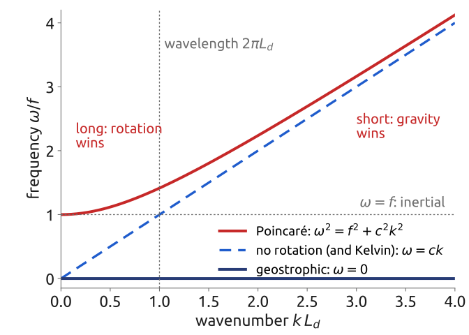
Rotation sets a lowest frequency, \(f\), and a length scale, \(L_d = \sqrt{gH}/f\)

(Vallis 2017, sec. 3.8; Cushman-Roisin and Beckers 2011, sec. 9.3)

Ask first: what happens to a very long wave when the Earth rotates? (It becomes an inertial oscillation: period 2 pi/f, 17 h.) Poincare waves: Poincare (1910, tides). Group velocity c^2 k/omega < c.

Gravity waves seen from space

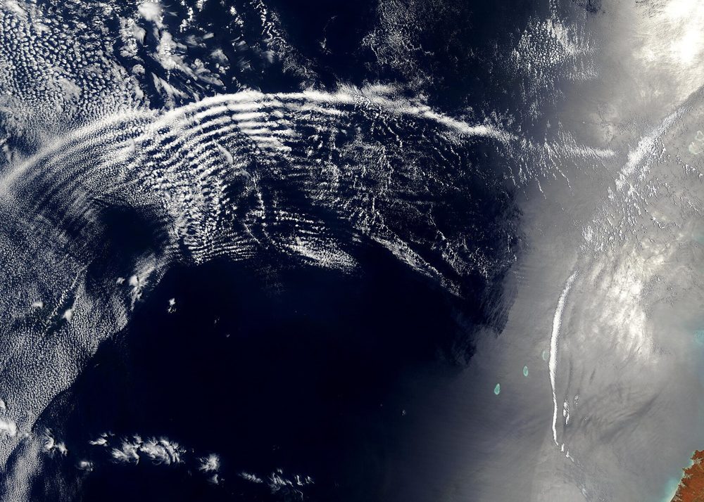
NASA, MODIS (Terra), 11 Nov 2003; public domain

Atmosphere, from space: arcs of wave clouds off Western Australia

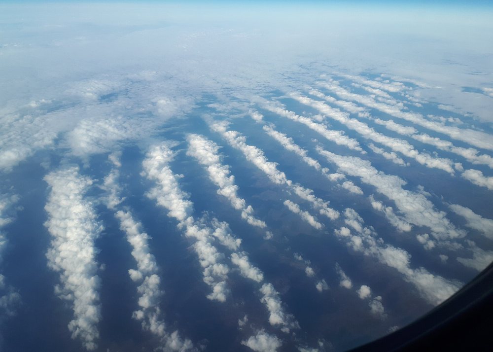
M. Häggström, 2018; CC BY-SA 4.0

From a plane: one band of cloud per crest, where the lifted air cools and its vapour condenses

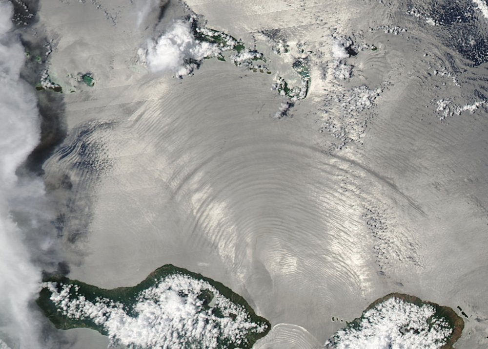
NASA, MODIS (Aqua), 1 Nov 2016; public domain

Ocean: internal waves set off by the tide in the Lombok Strait (Bali, Lombok below), seen in the sunglint. With \(g' \approx 0.02\) m/s², \(H = 100\) m: \(c = \sqrt{g'H} \approx 1.4\) m/s

Inside the atmosphere and the ocean gravity is reduced: slow internal gravity waves, km apart

From space: commons.wikimedia.org: File, NASA SVS 14445 · Plane: commons.wikimedia.org: File (another view) · Ocean: commons.wikimedia.org: File

Ask first: which wave is faster, the one at the sea surface or the one at the thermocline? (Surface: c = sqrt(gH), 200 m/s in a 4 km ocean; thermocline: g’ = g delta rho/rho0 = 0.02 m/s^2, c = 1.4 m/s for H = 100 m.) Rotation does not matter at these scales (km, minutes to hours). The clouds: internal gravity waves of the stratified air; the reddit link (ref line) is another plane view to show online (restoring force: buoyancy, frequency N). The shallow-water layer is the simplest model of both.

The deformation radius

\[L_d = \frac{\sqrt{gH}}{f}\]

how far a gravity wave travels in a time \(1/f\)

• One layer, full depth: thousands of km
• Stratified: \(L_d = NH/f\); first mode \(NH/(\pi f)\) (red band)
• Wider than \(L_d\), slower than a day: balanced

\(N\): buoyancy frequency (air \(10^{-2}\), sea \(2\times10^{-3}\) s\(^{-1}\)); \(H\): 10 km, 4 km; \(45^\circ\)N. Green: today’s gravity waves

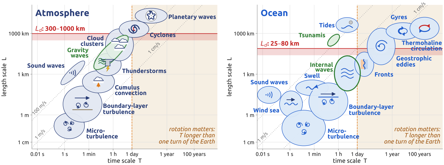
\(L_d\) sets the size of weather systems and ocean eddies: ocean “weather” is ten times smaller

(Vallis 2017, sec. 3.9; Cushman-Roisin and Beckers 2011, sec. 9.3)

Also called the Rossby radius. Stratified: c = NH (N = 1e-2, H = 10 km; ocean N = 2e-3, H = 4 km); the first vertical mode has c_1 = NH/pi (lecture 4) and L_1 = c_1/f: 300 km and 25 km; observed ocean radii: some tens of km at mid-latitudes, less at high latitudes, more near the equator. Ocean models must resolve such eddies: grids of a few km (lecture 9).

Kelvin waves (1/3): along a coast

A straight coast along \(y = 0\), fluid in \(y > 0\): no flow through the wall. Put \(v = 0\) everywhere in Laplace’s equations:

\[\frac{\partial u}{\partial t} = -g\frac{\partial\eta}{\partial x}, \qquad {\color{#1f5ccc}{f u = -g\frac{\partial\eta}{\partial y}}}, \qquad \frac{\partial\eta}{\partial t} + H\frac{\partial u}{\partial x} = 0\]

• First and third: a gravity wave along the coast, \(\eta = F(x - ct)\,G(y)\), \(u = (g/c)\,\eta\), \(c = \sqrt{gH}\)
• Second, across the coast: geostrophic, \(G' = -(f/c)\,G\), so \(G = e^{-y/L_d}\)
• The wave going the other way, \(x + ct\), would need \(e^{+y/L_d}\): it grows away from the coast, impossible

\[\eta = A\,e^{-y/L_d}\,F(x - ct), \qquad u = \frac{g}{c}\,\eta, \qquad v = 0\]

\(A\): amplitude; \(F\): any shape; \(L_d = c/f\)

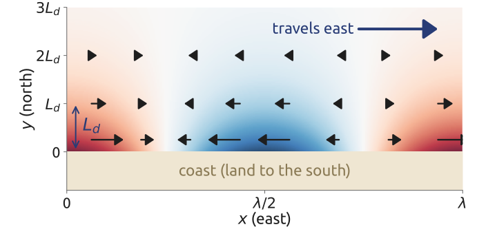
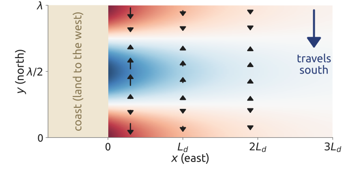
A wave trapped within \(L_d\) of the coast, with the coast on its right (northern hemisphere)

(Thomson 1880; Cushman-Roisin and Beckers 2011, sec. 9.2; Vallis 2017, sec. 3.8.3)

Thomson (Kelvin) 1880 (read 1879). Across the coast: f u = -g d(eta)/dy balance; along: a non-dispersive gravity wave, any shape, at c. Coast on the right: south coast, eastward; west coast, southward (bottom figure). Southern hemisphere: coast on the left.

Kelvin waves (2/3): around a basin, the tides

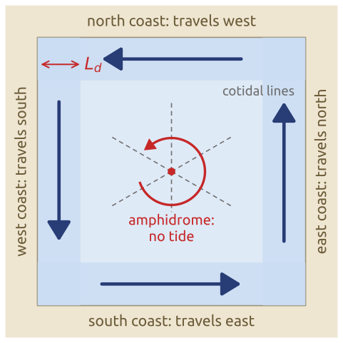
Northern hemisphere (southern: coast on the left, clockwise). \(L_d = \sqrt{gH}/f\) at \(45^\circ\)N: 200–300 km in a shelf sea 50–100 m deep, 1900 km in a 4 km deep ocean

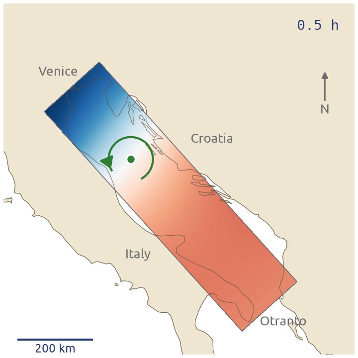
The M2 tide in an idealized Adriatic over one cycle (a linear shallow-water model): high water enters along the Croatian coast, reaches Venice and leaves along the Italian coast, around the amphidrome (green dot)

In a closed sea the Kelvin wave runs in along one coast and out along the other: an amphidrome

(Cushman-Roisin and Beckers 2011, secs. 9.2, 9.8)

Ask first: in a closed sea in the northern hemisphere, which way does the high tide go round? (Anticlockwise.) A closed sea (Adriatic, North Sea): the Kelvin waves along the coasts make an amphidrome, no tide at the centre, high water turning around it. The video: the model of notebook 06c (lecture 6), idealized, not observations (figures/src/tide-adriatic-video.py). Open oceans, many L_d wide: Kelvin and Poincare waves reflect and interfere (CR&B 9.8), and some amphidromes turn against the hemisphere rule (the global video with coloured dots is in the notes, figures/tide-amphidromes.mp4, if asked).

Kelvin waves (3/3): the equator as a coast

On the equatorial beta-plane \(f = \beta y\) changes sign at the equator. An eastward wave has the equator on its right in the north (\(f > 0\)) and on its left in the south (\(f < 0\)): both balances hold, \(\beta y\, u = -g\,\partial\eta/\partial y\)

\[u = G(x - ct)\,e^{-y^2/(2L_{eq}^2)}, \qquad \eta = \frac{H}{c}\,u, \qquad v = 0\]

\(G\): any shape; \(L_{eq} = (c/\beta)^{1/2}\): the equatorial deformation radius

• Eastward only, trapped within \(L_{eq}\) of the equator: \(L_{eq} \approx 1000\) km in the atmosphere (\(c = 25\) m/s), 300 km in the ocean (\(c = 2\) m/s)
• Seen in the stratosphere (zonal wavenumber 1, periods of 12–20 days), and coupled to convection as eastward-moving bands of tropical rain

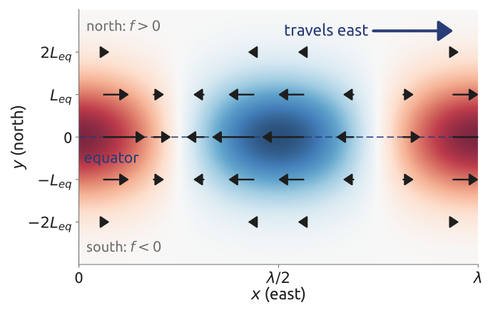
Shading: \(\eta\) (red high, blue low); arrows: \(u\)

Coast on the right in the north, on the left in the south: along the equator both mean east

(Matsuno 1966; Vallis 2017, sec. 8.2, eqs. 8.21, 8.57–8.63; Holton 2004, secs. 11.4.2, 12.5.3; Kiladis et al. 2009)

Matsuno (1966): the equatorial waves of shallow water on the beta-plane. Holton: Y_K = (2c/beta)^(1/2) = 1600 km for c = 30 m/s, the same scale up to sqrt 2. In the ocean the equatorial Kelvin waves carry the warm water east in El Nino (Vallis 22.7). Convectively coupled Kelvin waves: Matsuno’s structure, much of the tropical rainfall variability (Kiladis et al. 2009).

Kelvin waves in the air: rain patterns moving east

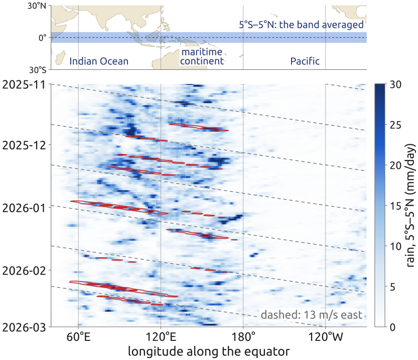
• Rain along the equator, day by day, November 2025 to February 2026: time runs down
• Streaks tilted to the right: the rain pattern moves east, from the Indian Ocean to the Pacific
• Red: the part moving east with periods of 2.5 to 30 days; measured speed 13 m/s
• As a Kelvin wave, \(c = \sqrt{gh}\) needs \(h = c^2/g \approx 17\) m: far from the 10 km of the atmosphere. Coupled to rain, the wave is slow
• Trade winds blow west, the rain pattern moves east: not one cloud travelling, but new clouds forming further east. Waves don’t carry air, they carry the pattern (in a wind \(U\), at \(U + c\))

ERA5 (Hersbach et al. 2020); contains modified Copernicus Climate Change Service information [2026]

Part of the tropical rain falls in patterns that travel east as equatorial Kelvin waves

(Matsuno 1966; Kiladis et al. 2009) · Data: cds.climate.copernicus.eu: ERA5 hourly data on single levels

Ask first: which way do the streaks go? (East: tilted right as time runs down.) Then: the trades blow west, how can the rain go east? Pattern vs parcels (air sloshes a few m/s); Doppler shift U + c, e.g. U = -5 m/s gives c = 18 m/s relative to the air (an example, not a measured mean). Same idea, reversed, in the Rossby slides: westward relative to an eastward jet. Speed from the data: lagged correlation of the filtered field, 10 degrees of longitude per day = 13 m/s (figures/src/kelvin-rain.py). The dry Kelvin wave of the whole troposphere would be much faster; coupled to convection the waves are slow (Kiladis et al. 2009: their scales do not match the linear theory of dry waves; their horizontal structure is Matsuno’s). Equivalent depth: the vertical-modes lecture. Plot cut at 90 W: further east, a fixed column of rain over the Pacific coast and Andes of Colombia and Ecuador (ERA5 about 14 mm/day at 77-79 W), not a wave.

Rossby waves (1/4): the mechanism

\[\Big(\frac{\partial}{\partial t} + U\frac{\partial}{\partial x}\Big)\zeta' + \beta v' = 0\] \[\zeta' = \nabla^2\psi', \qquad v' = \frac{\partial\psi'}{\partial x}\]

\(U\): eastward wind; \(\psi'\), \(\zeta'\), \(v'\): the wave’s streamfunction, vorticity, northward velocity; \(\beta = df/dy\)

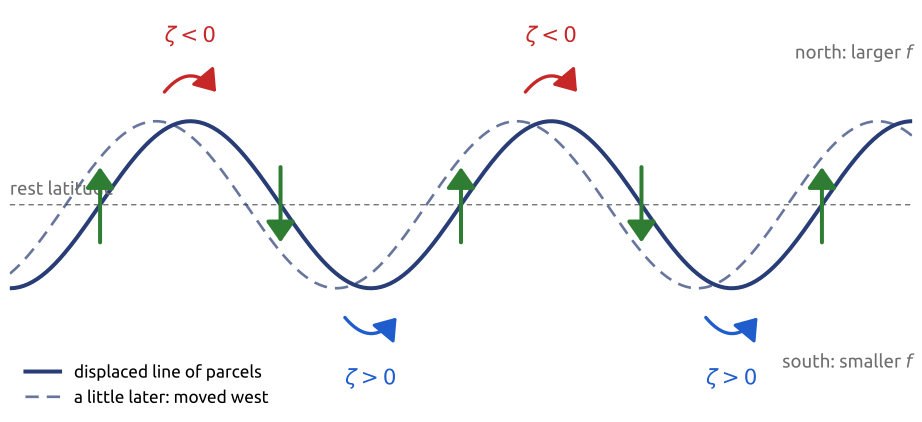
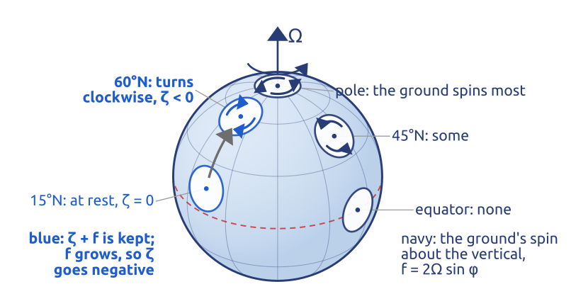
• Parcels keep \(\zeta + f\): moved north (larger \(f\)), \(\zeta < 0\); moved south, \(\zeta > 0\)
• They push their neighbours north west of a crest, south east of it: the pattern moves west

The variation of \(f\) with latitude (\(\beta v'\)) makes waves that travel west relative to the air

(Vallis 2017, sec. 6.4.2, eq. 6.57; Cushman-Roisin and Beckers 2011, sec. 9.4)

D(zeta + f)/Dt = 0 linearized about a uniform eastward wind U: the wind carries zeta’ (U d/dx), the parcel’s change of f appears as beta v’. Restoring “force”: the PV gradient beta. Same argument with any background PV gradient (topographic Rossby waves, ridge slide).

Rossby waves (2/4): wind east, waves west

A plane wave \(\psi' \propto e^{i(kx + ly - \omega t)}\): \(\zeta' = -K^2\psi'\), \(v' = ik\psi'\), \(K^2 = k^2 + l^2\)

\[\omega = Uk - \frac{\beta k}{K^2}, \qquad \frac{\omega}{k} = \underbrace{U}_{\text{carried east}}\;\underbrace{-\;\frac{\beta}{K^2}}_{\text{drift west, through the air}}\]

• Through the air always west; over the ground, \(U - \beta/K^2\):
  • long waves, \(K^2 < \beta/U\): west
  • \(K^2 = \beta/U\), \(2\pi\sqrt{U/\beta} \approx 6000\) km: stand still
  • short waves, \(K^2 > \beta/U\): east
• Packets: \(c_g = \partial\omega/\partial k = U + \beta(k^2 - l^2)/K^4\), faster east than the troughs
• With a free surface, no wind: \(\omega = -\beta k/(K^2 + L_d^{-2})\); ocean long waves, a few cm/s: years to cross a basin

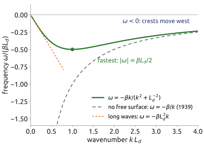
Rossby waves: carried east by the wind, always drifting west through the air

(Rossby and collaborators 1939; Vallis 2017, sec. 6.4.2, eqs. 6.60–6.62, 6.66)

Ask first: in an eastward wind, can a Rossby wave stand still? (Yes: U = beta/K^2; 4-5 waves around 45 N, as on 500 hPa maps.) U = 15 m/s, beta = 1.6e-11 at 45 N: 6000 km. The figure: no wind, finite L_d (the ocean case). With a free surface AND a wind, the wind also tilts the surface and changes the PV gradient (beta + U/L_d^2): not a pure Doppler shift (Vallis 6.66-6.68); the barotropic case keeps it simple. Group velocity: Vallis 6.62-6.63, c_g = c + 2 beta k^2/K4: packets always faster east than troughs.

Rossby waves (3/4): reading the diagram

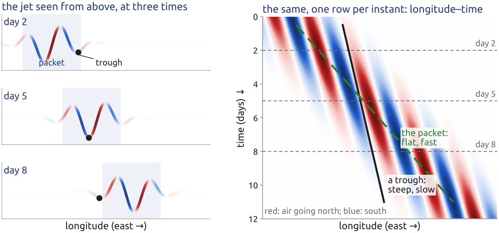
• Each row is the jet at one instant, time down: standing still, a vertical stripe; moving east, tilted right, flatter = faster

• A trough (a low-pressure system) sits where blue turns to red, going east: steep, slow. The packet (green): flat, fast

In a longitude–time diagram, speed is slope: troughs and packet move at different speeds

(Hovmöller 1949; Vallis 2017, sec. 6.4.2) · Schematic: troughs at 5 m/s, packet at 19 m/s

Ask first: on the right, which line is a trough? The boundary where blue (air going south, into the dip) turns to red (going north, out of it), going east; the trough itself is white (v = 0 at its bottom). A trough grows as the packet arrives and fades after it (the dot on the left). Schematic, not data (figures/src/ hovmoller-reading.py): a Gaussian packet of zonal wavenumber 6, troughs at c = 5 m/s, packet at c_g = 19 m/s, about the August 2002 values of the next slide. The colour is v, the northward wind: blue to red going east is a trough (southward dip). Hovmoller (1949) drew these by hand. The packet is “downstream development”: new troughs grow ahead of it, old ones decay behind (a pattern of patterns, as with the Kelvin rain).

Rossby waves (4/4): theory against data

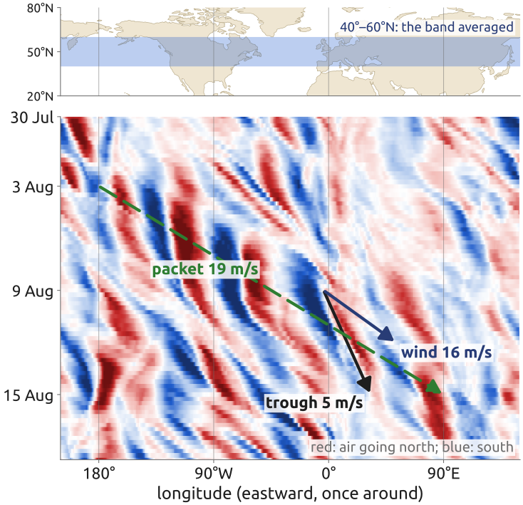
m/s, east	data	\(U_{500}\)	\(U_{250}\)
wind \(U\)	8–16	8	16
troughs \(U - \beta/k^2\)	3–5	1	9
packet \(U + \beta/k^2\)	19	15	22

Theory with \(U\) at 500 or 250 hPa; wavenumber 6 at 50°N (4300 km): \(\beta/k^2 \approx 7\) m/s

• The jet in August 2002, before the Elbe flood
• Troughs (low-pressure systems; blue to red, going east) crawl: carried at \(U\), pulled back at \(\beta/k^2\)
• The packet runs at \(U + \beta/k^2\): new troughs grow ahead of it, faster than troughs and wind
• Data between the two levels: the wave feels the whole troposphere

ERA5 (Hersbach et al. 2020); contains modified Copernicus Climate Change Service information [2026]

The wind carries the troughs east, \(\beta\) pulls them west: troughs crawl, packets run

(Wirth et al. 2018, 1972; Vallis 2017, sec. 6.4.2) · Data: cds.climate.copernicus.eu: ERA5 hourly data on pressure levels

The case of lecture 1 (Elbe flood), now with numbers. Wind: mean u, 40-60 N, 3-15 Aug, 15.6 m/s at 250 hPa, 8.2 at 500 hPa. Troughs: the one followed in lecture 1, 5 m/s; all troughs by lagged correlation, 3 m/s (same at both levels). Packet: Wirth et al. 18.6 m/s (180 on 3 Aug to 90 E on 15 Aug); hemisphere-wide envelope 12-15 m/s. Dominant zonal wavenumber 6 at both levels. Barotropic with l = 0 is rough (the jet’s own PV gradient, the vertical structure); the point is the order: troughs < wind < packet. figures/src/rossby-2002-theory.py prints all numbers.

Fast and slow: the four waves

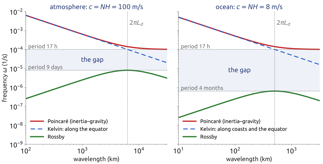
• Fast: Poincaré, periods under 17 h; Kelvin at \(c\), along walls only

• Slow: Rossby, over 9 days in the air, 4 months in the sea

The weather lives in the slow branch; the fast branch limits the time step

(Vallis 2017, sec. 3.8 and sec. 6.4; Gill 1982)

Stratified, c = NH: air N = 1e-2, H = 10 km, c = 100 m/s, L_d = 1000 km: Rossby periods >= 9 days; sea N = 2e-3, H = 4 km, c = 8 m/s, L_d = 80 km: >= 4 months (slowest Rossby frequency beta L_d/2). Kelvin dashed through the gap: they exist at any frequency, but only along walls. How does the flow get into the slow branch? Adjustment, next. Time step: lecture 5.

Geostrophic adjustment (1/3): release a step

\[\begin{aligned} \frac{\partial u}{\partial t} - {\color{#c62828}{f v}} &= -g\frac{\partial\eta}{\partial x}\\ \frac{\partial v}{\partial t} &= -{\color{#c62828}{f u}}\\ \frac{\partial\eta}{\partial t} + H\frac{\partial u}{\partial x} &= 0 \end{aligned}\]

Start: \(\eta = \pm\eta_0\), \(u = v = 0\)

• \(f = 0\): a wave equation; fronts leave both ways at \(c = \sqrt{gH}\); between them water flows from high to low
• \(f > 0\): \(\partial v/\partial t = -fu\) turns that current along the step: geostrophic, Rossby (1938)

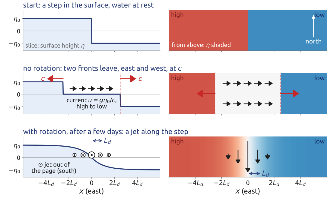
Rotation turns the current along the step: part of the step stays, balanced

(Rossby 1938; Vallis 2017, sec. 3.9, eqs. 3.136–3.142)

Ask first: with rotation, what does the step become after a few days? Sketch it from above. Vallis 3.139, 3.142 (f = 0): eta = -(eta0/2)[sgn(x + ct) + sgn(x - ct)], u = g eta0/c between the fronts; like a dam break. f > 0: the cross-step current is turned by Coriolis (red terms) into a jet along the step, southward with the high to the west (high on its right). The adjustment leaves inertial oscillations (not drawn). Rossby (1937, 1938); Gill 1982 §7.2. Next slide: how much stays, from PV.

Geostrophic adjustment (2/3): what is kept

From the equations of the step (with \(f = f_0\)):

\[\begin{aligned} &\textbf{1.}\;\; \frac{\partial v}{\partial t} = -f_0 u &&\xrightarrow{\;\partial/\partial x\;}\quad \frac{\partial \zeta}{\partial t} = -f_0\,\frac{\partial u}{\partial x}, \qquad \zeta = \frac{\partial v}{\partial x}\\[6pt] &\textbf{2.}\;\; \frac{\partial\eta}{\partial t} + H\frac{\partial u}{\partial x} = 0 &&\xrightarrow{\phantom{\;\partial/\partial x\;}}\quad \frac{\partial u}{\partial x} = -\frac{1}{H}\frac{\partial\eta}{\partial t}\\[6pt] &\textbf{3.}\;\; \text{put 2 in 1:} &&\phantom{\xrightarrow{\;\partial/\partial x\;}}\quad \frac{\partial\zeta}{\partial t} = \frac{f_0}{H}\frac{\partial\eta}{\partial t} \end{aligned}\]

\[\frac{\partial q}{\partial t} = 0, \qquad q = \zeta - \frac{f_0\,\eta}{H}\]

At the start \(\zeta = 0\) and \(\eta = -\eta_0\,\mathrm{sgn}(x)\), so \(q = \dfrac{f_0\eta_0}{H}\,\mathrm{sgn}(x)\) for ever, whatever the waves do

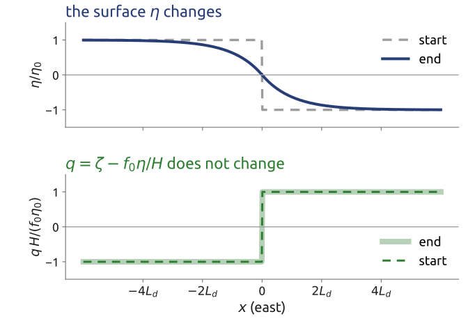
The waves change \(\eta\) and the flow, but not \(q\): the step’s potential vorticity is its memory

(Vallis 2017, sec. 3.9.2, eqs. 3.143–3.146 and Fig. 3.10)

The linear version of (zeta + f)/h kept by each column (Vallis 3.145: Q ~ (f0 + q)/H). Here q is fixed in space, not only following parcels: the advection of q is quadratic, dropped. The non-rotating case also keeps q (= zeta = 0), but that tells nothing: with f0 the constraint is strong.

Geostrophic adjustment (3/3): the balanced state

At the end the flow is steady, \(\partial/\partial t = 0\):

\[\begin{aligned} &\textbf{1.}\;\; \text{geostrophic:} && f_0 v = g\,\frac{\partial\eta}{\partial x}\\[4pt] &\textbf{2.}\;\; \text{so} && \zeta = \frac{\partial v}{\partial x} = \frac{g}{f_0}\frac{\partial^2\eta}{\partial x^2}\\[4pt] &\textbf{3.}\;\; \text{into the kept } q: && \frac{g}{f_0}\frac{\partial^2\eta}{\partial x^2} - \frac{f_0}{H}\,\eta = \frac{f_0\eta_0}{H}\,\mathrm{sgn}(x) \end{aligned}\]

\[\frac{\partial^2\eta}{\partial x^2} - \frac{\eta}{L_d^2} = \frac{\eta_0}{L_d^2}\,\mathrm{sgn}(x) \;\Rightarrow\; \eta = -\eta_0\,\mathrm{sgn}(x)\big(1 - e^{-|x|/L_d}\big)\]

\(L_d = \sqrt{gH}/f_0\) (step 3 times \(f_0/g\)); jet: \(v = -\dfrac{g\eta_0}{f_0L_d}\,e^{-|x|/L_d}\)

• Only one third of the energy released stays in the jet; two thirds leave as waves

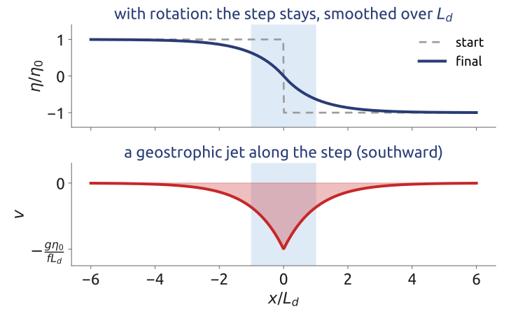
Rotating fluids adjust by radiating gravity waves: why the large-scale flow is geostrophic

(Rossby 1938; Vallis 2017, sec. 3.9, eqs. 3.147–3.151; Gill 1982, sec. 7.2)

PV conservation and geostrophy alone give the final state: no need to follow the waves (Vallis 3.147-3.151). Vallis writes it with psi = g eta/f0: (d2/dx2 - 1/L_d^2) psi = q, the same equation times g/f0. Check the solution on the board: x > 0, eta = -eta0 + eta0 e^(-x/L_d). Far away eta -> -eta0 sgn x, the step; near x = 0 it is smoothed. Richardson’s problem in reverse: his initial state was unbalanced.

Notebook Waves and adjustment

Notebook 03b (open in Colab · download): waves and adjustment in rotating shallow water, on a computer.

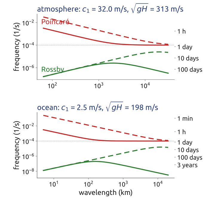
Red: Poincaré; green: Rossby. Solid: first vertical mode; dashed: external mode

1. Dispersion relations: Poincaré waves above \(f\), Rossby below, a gap between; the first vertical mode (solid) against the whole depth moving together (dashed)
2. A bump without rotation: two gravity waves leave at \(\sqrt{gH}\)
3. With rotation: what leaves and what stays, for narrow and wide bumps ❗ 3.1
4. Rossby’s step: watch the adjustment; the jet, of width \(L_d\) ❗ 4.1
5. An eddy on the beta-plane drifts west

Predict, run, explain: write down what you expect before each run

A computer solves the shallow water equations: watch the waves leave and the balance stay

(Rossby 1938; Vallis 2017, secs. 3.8–3.9)

In class, 15 min: sections 2 to 4 (a bump without and with rotation; Rossby’s step); sections 1 and 5 at home. The solver is a black box today; it is opened in lecture 5. If time is short: section 4 only.

What the notebook showed

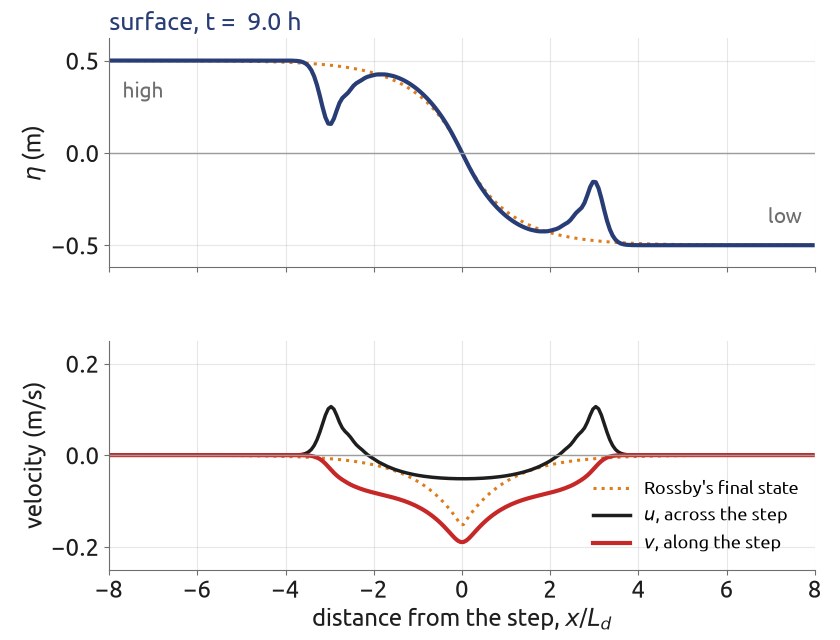
Rossby’s step, three days; dotted: his final state

• Without rotation a bump leaves as two gravity waves, at \(\sqrt{gH}\); nothing stays
• With rotation the water first runs from high to low, \(u\); the Coriolis force turns it along the step, \(v\), within half an inertial period, \(\pi/f \approx 9\) h
• It overshoots, oscillates at \(2\pi/f\), and settles on Rossby’s jet, of width \(L_d\): one third of the energy stays
• Bumps wider than \(L_d\) stay; narrower ones are radiated away

Large-scale disturbances stay balanced; small ones are shaken off as waves

(Vallis 2017, sec. 3.9; Cushman-Roisin and Beckers 2011, sec. 15.2)

The step is smoothed over 50 km for the video: a sharp step makes grid ripples at any resolution (the notebook’s aside). The atmosphere is forced at large scales (heating): it stays near balance. Weather prediction: initial data must be balanced, or the model makes spurious gravity waves (initialization).

Quasi-geostrophy (1/2): from shallow water

Start: shallow water in vorticity form (the vorticity and mass equations), flat bottom, \(h = H + \eta\), \(f = f_0 + \beta y\): \(\;\dfrac{D(\zeta + f)}{Dt} = -(\zeta + f)\,\nabla\cdot\mathbf{u},\quad \dfrac{D\eta}{Dt} = -(H + \eta)\,\nabla\cdot\mathbf{u}\)

Assume: \(Ro = U/(f_0L) \ll 1\); scales near \(L_d\), so \(\eta \ll H\); \(\beta L \ll f_0\).

\[\begin{aligned} &\textbf{1.}\ \text{leading order, geostrophic:} && \mathbf{u}_g = \mathbf{k}\times\nabla\psi, \quad \psi = \frac{g\eta}{f_0}, \quad \zeta = \nabla^2\psi\\[2pt] &\textbf{2.}\ \text{vorticity, stretching by } f_0 \text{ only:} && \frac{D_g}{Dt}(\zeta + \beta y) = -f_0\,\nabla\cdot\mathbf{u}\\[2pt] &\textbf{3.}\ \text{mass, } \eta \ll H \text{, eliminates } \nabla\cdot\mathbf{u}: && \nabla\cdot\mathbf{u} = -\frac{1}{H}\frac{D_g\eta}{Dt} \quad\Longrightarrow\quad \frac{D_g}{Dt}\Big(\zeta + \beta y - \frac{f_0\eta}{H}\Big) = 0 \end{aligned}\]

\[\frac{\partial q}{\partial t} + J(\psi, q) = 0, \qquad q = \nabla^2\psi - \frac{\psi}{L_d^2} + \beta y\]

\(J(\psi, q) = \partial_x\psi\,\partial_y q - \partial_y\psi\,\partial_x q = \mathbf{u}_g\cdot\nabla q\); \(D_g/Dt = \partial_t + \mathbf{u}_g\cdot\nabla\); \(f_0\eta/H = \psi/L_d^2\)

• The flow is geostrophic, but it evolves through the small divergence that step 3 eliminates
• \(q\) is the shallow-water \((\zeta + f)/h\) to first order: the adjustment’s \(q\), plus \(\beta y\)

Quasi-geostrophy: geostrophy for the flow, potential vorticity for its evolution

(Charney 1948; Vallis 2017, sec. 5.3.1, eqs. 5.56–5.69)

Step 2: curl of the momentum equation at first order in Ro (Vallis 5.59-5.60); stretching by zeta is a factor Ro smaller. Step 3: the mass equation at first order (5.58). Assumptions as in Vallis 5.3 (i)-(iv); eta/H ~ Ro (L/L_d)^2. The same q (without beta) kept the step’s memory in the adjustment.

Quasi-geostrophy (2/2): properties and practice

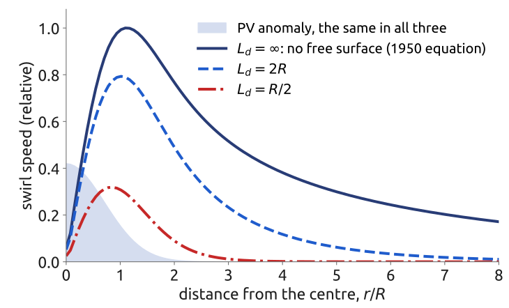
The same PV anomaly, three deformation radii: the free surface confines its flow to a few \(L_d\)

• One unknown, \(q\). Each time step: invert \(\;(\nabla^2 - L_d^{-2})\,\psi = q - \beta y\;\) for \(\psi\) (an elliptic problem: the figure), then advect \(q\) with \(\mathbf{u}_g\)
• No gravity waves: linearized, only the Rossby waves, \(\omega = -\beta k/(K^2 + L_d^{-2})\). The time step is set by the wind, \(U\), not by \(c\): ten times longer or more
• Conserved: energy \(\frac{1}{2}\int(|\nabla\psi|^2 + \psi^2/L_d^2)\,dA\), kinetic plus potential, and enstrophy \(\frac{1}{2}\int q^2\,dA\). Kinetic/potential \(\sim (L_d/L)^2\)
• Valid for \(Ro \ll 1\), scales near \(L_d\), \(\beta L \ll f_0\): not near the equator, not at fronts
• Practice: Charney (1948) for the stratified atmosphere; the first computer forecasts (1950s); today theory and idealized models. \(L_d \to \infty\): the 1950 equation

Quasi-geostrophy keeps the slow, balanced flow: one PV equation, inverted for \(\psi\) at each step

(Charney 1948; Vallis 2017, secs. 5.3, 5.6; Cushman-Roisin and Beckers 2011, Ch. 16; Lynch 2008b)

Ask first: the same PV blob in the ocean (L_d 30 km) and in the atmosphere (1000 km): which drives the wider flow? Energy: multiply the equation by -psi and integrate (Vallis 5.159 for the stratified case); enstrophy by q: an invariant of the QG limit (Vallis 5.3.3). Operational forecasts: quasi-geostrophic models in the 1950s, primitive equations from the 1960s (Lynch 2008).

Barotropic vorticity (1/2): no divergence

Start: shallow water in vorticity form, \(\;\dfrac{D(\zeta + f)}{Dt} = -(\zeta + f)\,\nabla\cdot\mathbf{u}\)

1. Rigid lid, flat bottom: \(h = H\), so mass gives \(\nabla\cdot\mathbf{u} = 0\). Fair when the surface hardly moves: \(\eta/H \sim Ro\,L^2/L_d^2\), small for \(L \ll L_d\)
2. Then \(D(\zeta + f)/Dt = 0\): each column keeps its absolute vorticity (Rossby 1939)
3. No divergence: a streamfunction, \(u = -\partial_y\psi\), \(v = \partial_x\psi\), \(\zeta = \nabla^2\psi\), and \(\mathbf{u}\cdot\nabla = J(\psi,\cdot)\)

\[\frac{\partial}{\partial t}\nabla^2\psi + J\big(\psi,\ \nabla^2\psi + f\big) = 0\]

The quasi-geostrophic equation with \(L_d \to \infty\); here \(\psi\) comes from \(\nabla\cdot\mathbf{u} = 0\), not from geostrophy

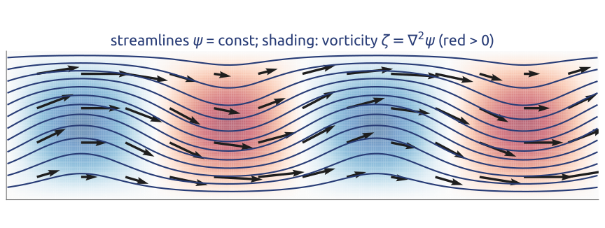
With no divergence, shallow water reduces to one equation for one unknown, \(\psi\)

(Vallis 2017, secs. 3.1.3, 5.3; Rossby and collaborators 1939)

Exact under the rigid lid: no expansion in Ro needed. Why a rigid lid is fair: external L_d of the atmosphere ~3000 km, systems of 1000 km have L^2/L_d2 ~ 0.1. The same equation is QG with L_d -> infinity (previous slide).

Barotropic vorticity (2/2): the 1950 forecast

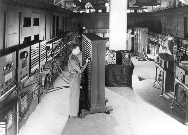
The ENIAC. U.S. Army photo, public domain

\[\frac{\partial}{\partial t}\nabla^2\psi + J(\psi,\ \nabla^2\psi + f) = 0\]

• No \(\eta\), no gravity waves: only Rossby waves, so long time steps (3 h)
• Each step: a Poisson problem, \(\nabla^2\psi = \zeta\)
• Charney, Fjørtoft and von Neumann (1950): the first successful computer forecast

The 1950 equation is shallow water with the fast waves filtered out: the ENIAC forecast, derived

(Charney et al. 1950; Lynch 2008a) · Photo: commons.wikimedia.org: Classic shot of the ENIAC

The ENIAC story: lecture 1. u . grad zeta = J(psi, zeta) for u = k x grad psi = (-psi_y, psi_x); the order matters, J(zeta, psi) = -J(psi, zeta). Richardson kept the gravity waves and his step was too long; Charney filtered them. Spectral methods (lecture 7) make the Poisson problem trivial.

Ekman layer (1/4): friction near the surface

Geostrophy: Coriolis against pressure. Under the wind: Coriolis against friction (viscous, with an eddy viscosity \(\nu_E \approx 10^{-2}\) m²/s). Steady, f-plane, uniform stress \(\boldsymbol{\tau}\), deep ocean:

\[f\,\mathbf{k}\times\mathbf{u} = {\color{#1f5ccc}{\nu_E\,\frac{\partial^2\mathbf{u}}{\partial z^2}}}\]

\(f\): Coriolis parameter; \(\mathbf{u}(z)\): horizontal velocity; \(\mathbf{k}\): upward unit vector; \(\rho_0\): density of the water

\(-fv = \nu_E u_{zz}\), \(\;fu = \nu_E v_{zz}\); \(\;\rho_0\nu_E\,\partial_z\mathbf{u} = \boldsymbol{\tau}\) at \(z = 0\); \(\;\mathbf{u} \to 0\) deep

• Whole depth: \(Ek = \nu_E/(fH^2) \approx 10^{-5}\)
• Friction acts within a few \(d = \sqrt{2\nu_E/f} \approx 14\) m

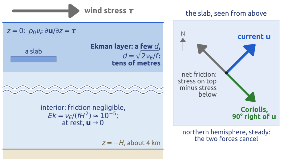
Coriolis against friction: only in a thin layer under the wind, where the shear is strong

(Cushman-Roisin and Beckers 2011, secs. 8.2, 8.6; Vallis 2017, sec. 5.7.1)

Ask first: the wind blows north (northern hemisphere): which way does the water at 10 m go? (Slide 3: about 86° right of the wind, nearly east, at half the surface speed.) nu_E: eddy viscosity, 10^4 times the molecular one. Ek is small, but friction has the highest derivative: a boundary layer (Prandtl). Ekman (1905), for Nansen’s ice (lecture 1). Friction: lecture 2’s viscous term.

Ekman layer (2/4): one complex equation

One complex number for the velocity, east the real axis, north the imaginary; \(i(u + iv) = -v + iu\):

\[W = u + iv, \qquad \mathbf{k}\times\mathbf{u} \;\leftrightarrow\; iW\]

\[\nu_E\,\frac{d^2W}{dz^2} = if\,W \;\Rightarrow\; W = A\,e^{{\color{#1f5ccc}{(1+i)}}z/d}\]

\(A\): a complex constant, set by the wind at the surface

• Try \(e^{\lambda z}\): \(\lambda^2 = if/\nu_E = 2i/d^2\), and \((1+i)^2 = 2i\)
• Keep \(\lambda = (1+i)/d\): it decays as \(z \to -\infty\)
• \(e^{(1+i)z/d} = e^{z/d}\,e^{iz/d}\): weaker, and turned

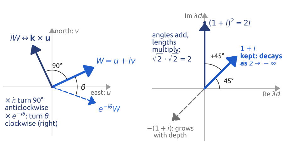
Each \(d\) down: \(e\) times weaker, and turned 57° clockwise (northern hemisphere)

(Holton 2004, sec. 5.3.4, eqs. 5.29–5.31; real form: Cushman-Roisin and Beckers 2011, sec. 8.3; Vallis 2017, sec. 5.7.3)

Real and imaginary parts of nu_E W’’ = i f W give back the pair of slide 1; the complex form is Holton’s (sec. 5.3.4). Cushman-Roisin & Beckers solve the real pair: nu_E^2 lambda^4 + f^2 = 0. Below the surface z < 0: e^{iz/d} turns clockwise as z decreases, one radian per d.

Ekman layer (3/4): the surface condition, 45°

At \(z = 0\), with the stress as a complex number too, \(\tau = \tau_x + i\tau_y\):

\[\begin{aligned} \rho_0\nu_E\,\frac{dW}{dz}(0) = \tau \;\Rightarrow\; A &= \frac{\tau d\,(1-i)}{2\rho_0\nu_E}\\ &= \frac{\sqrt{2}\,\tau}{\rho_0 fd}\,{\color{#1f5ccc}{e^{-i\pi/4}}} \end{aligned}\]

• \(e^{-i\pi/4}\): surface current 45° right of the wind (northern hemisphere; left in the southern)
• Deeper: weaker as \(e^{z/d}\), turning clockwise: the Ekman spiral
• At \(z = -\pi d\): 4 %, against the surface current

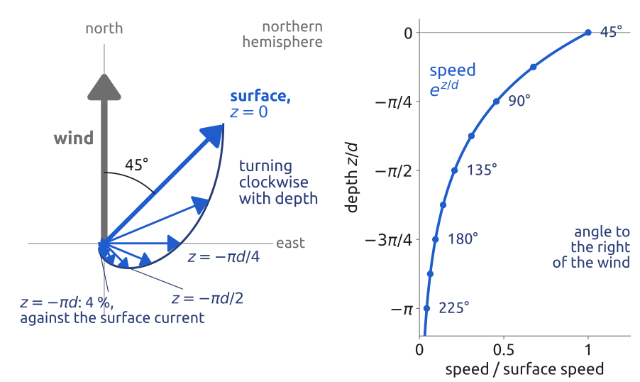
45° right of the wind at the surface, weaker and further right below (northern hemisphere)

(Ekman 1905; Cushman-Roisin and Beckers 2011, sec. 8.6; Vallis 2017, sec. 5.7.4)

Ask-first answer: 10 m is z/d = 0.7 rad (41°) down: 86° right of the wind, half the speed. Surface speed sqrt(2) tau/(rho0 f d): about 10 cm/s for tau = 0.1 N/m². Observed angles are smaller (5–20°): the eddy viscosity is not constant (Cushman-Roisin & Beckers §8.7).

Ekman layer (4/4): transport and pumping

Integrate \(\nu_E W'' = ifW\) over the layer: \(M = \int_{-\infty}^{0} W\,dz\) is the volume transport per unit width (m²/s), \(\mathbf{M}_E\) as a vector:

\[\begin{aligned} ifM &= \nu_E\big[W'\big]_{-\infty}^{0} = \frac{\tau}{\rho_0}\\ \Rightarrow\; M &= \frac{-i\tau}{\rho_0 f} \;\Leftrightarrow\; \mathbf{M}_E = \frac{\boldsymbol{\tau}\times\mathbf{k}}{\rho_0 f} \end{aligned}\]

• 90° right of the wind (northern hemisphere), whatever \(\nu_E\)
• Integrate \(\nabla\cdot\mathbf{u} + \partial_z w = 0\) over the layer:

\[w_E = \nabla\cdot\mathbf{M}_E = {\color{#1f5ccc}{\mathbf{k}\cdot\nabla\times\frac{\boldsymbol{\tau}}{\rho_0 f}}}\]

But: the squashed columns, how do they move? Sverdrup (1947).

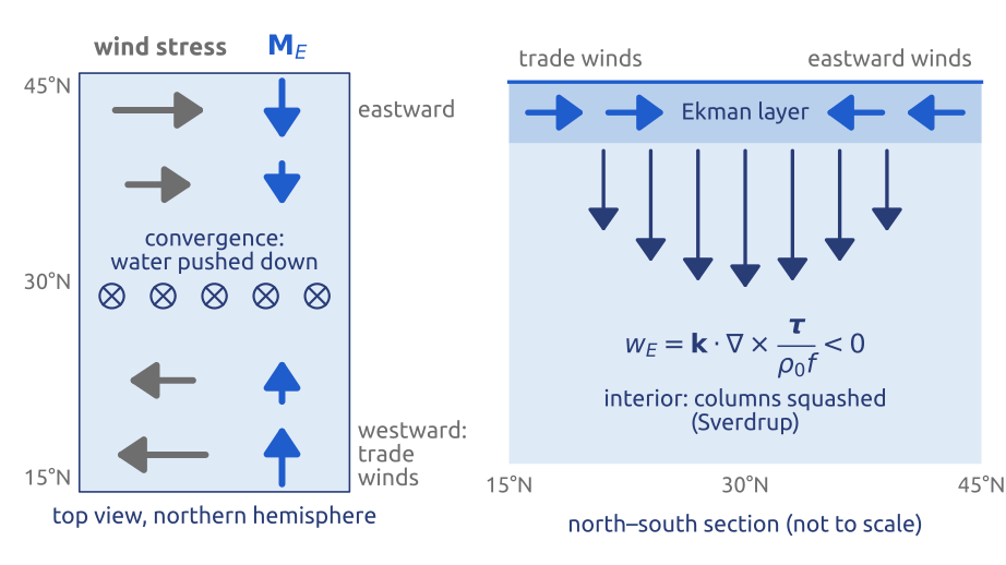
The transport does not depend on the friction; where it converges, it pumps water down

(Vallis 2017, sec. 5.7.2; Cushman-Roisin and Beckers 2011, sec. 8.6)

Lecture 1 gave the 90° from a force balance; here it is exact. -i turns 90° clockwise: -iW is u x k. Subtropical gyres: w_E about -1e-6 m/s, 30 m a year (Vallis §20.5). Next: Sverdrup, the squashed columns keep (zeta + f)/h by drifting south.

Sverdrup (1947): the wind drives the gyres

The barotropic vorticity equation, now forced by the curl of the wind and with weak bottom friction:

\[\frac{\partial\zeta}{\partial t} + J(\psi, \zeta) + \beta v = \frac{\mathbf{k}\cdot\nabla\times\boldsymbol{\tau}}{\rho_0 H} - r\zeta\]

Steady, slow and wide: only \(\beta v\) and the wind are left. With \(V = Hv\):

\[\beta V = \frac{\mathbf{k}\cdot\nabla\times\boldsymbol{\tau}}{\rho_0}\]

\(\boldsymbol{\tau}\): wind stress; \(V\): northward transport per unit width; \(H\): depth; \(r\): bottom friction rate; \(J(\psi, \zeta) = \mathbf{u}\cdot\nabla\zeta\), the advection of \(\zeta\), \(\psi\) the streamfunction

• Northern hemisphere, subtropics: Ekman pumping squashes the columns; to keep \((\zeta + f)/h\) they drift south
• \(\tau \approx 0.1\) N/m² over 1000 km: \(V \approx 5\) m²/s, 25 Sv across 5000 km
• Return flow narrow and fast, on the western side: the Gulf Stream (Stommel 1948)

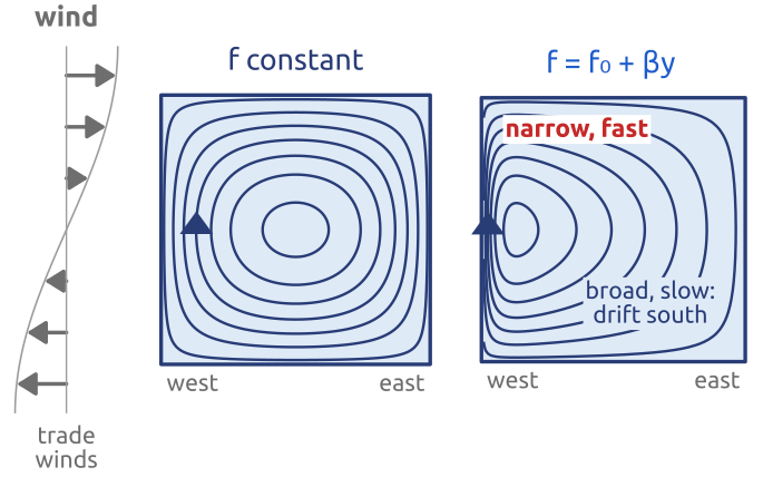
The 1950 equation, forced by the wind: the same \(\beta\) drives the ocean gyres

(Sverdrup 1947; Stommel 1948; Vallis 2017, secs. 19.1.2–19.1.3, eqs. 19.8, 19.20)

Vallis 19.8: D zeta/Dt + beta v = F; Sverdrup 19.20: beta v = curl of tau/(rho0 H) when friction is small (r zeta much smaller than beta v). Equivalently, beta V_g = f w_E for the geostrophic interior (Vallis 19.1.2); with the Ekman transport added, beta V = curl tau/rho0 exactly. 1 Sv = 1e6 m^3/s. Gulf Stream about 30 Sv at Florida. Stommel’s figure from the history lecture (bottom friction, r).

Key points

1. Thin and slow: hydrostatic (\(\partial p/\partial z = -\rho g\)) and nearly geostrophic (\(Ro \ll 1\))
2. Shallow water: \(\dfrac{D\mathbf{u}}{Dt} + f\mathbf{k}\times\mathbf{u} = -g\nabla\eta\), \(\;\partial_t h + \nabla\cdot(h\mathbf{u}) = 0\); linear: Laplace’s tidal equations
3. Potential vorticity \((\zeta + f)/h\) is kept by each column: depth and latitude steer the flow
4. Waves: gravity \(c = \sqrt{gH}\); Poincaré \(\omega^2 = f^2 + c^2K^2\); Kelvin, trapped at coasts and the equator, one way only
5. Rossby waves: \(\omega/k = U - \beta/K^2\), carried east by the wind, drifting west through the air; \(L_d = \sqrt{gH}/f\)
6. Adjustment: imbalance leaves as gravity waves; what is wider than \(L_d\) stays, balanced
7. Quasi-geostrophy: one potential vorticity, inverted for \(\psi\); with no divergence, the 1950 equation
8. Ekman: transport \(90^\circ\) right of the wind (northern hemisphere); its pumping, with \(\beta\), drives the gyres (Sverdrup)

Notebooks: 03a (open in Colab · download), exercise 1 comes back there; 03b (open in Colab · download), the waves and the adjustment.

A thin rotating layer of fluid: balance, potential vorticity and the waves of weather

Reading: (Vallis 2017, secs. 2.3–2.4, 2.7–2.8, 3.1, 3.7–3.9, 5.3, 5.7, 6.4, 8.2, 19.1; Cushman-Roisin and Beckers 2011, Ch. 7–9, 16)

Next lecture’s warm-up asks about these. Next: the vertical, so far averaged away (one layer) or balanced away (hydrostatic): buoyancy, internal waves, convection, mountains (lecture 4). Then how to compute these equations on a grid, with fast waves that limit the time step; why Richardson’s step failed and the ENIAC’s worked (lecture 5).