November 2026 · Politecnico di Milano

The vertical slice: buoyancy, convection and mountain waves

Atmosphere and Ocean Dynamics — Lecture 4

Prof. Dr. Pedro da Silva Peixoto

Applied Mathematics
Instituto de Matemática e Estatística
Universidade de São Paulo

Visiting Professor at MOX Lab
Politecnico di Milano

Warm-up

1. Why can large-scale models replace the vertical momentum equation by \(\partial p/\partial z = -\rho g\)? When would that fail?
2. Rossby waves: \(\omega/k = U - \beta/K^2\). Which way do they drift through the air? What makes them oscillate?
3. In geostrophic adjustment, what stays balanced, and what leaves as gravity waves?
4. A stratified ocean, \(N = 2\times10^{-3}\) s\(^{-1}\), \(H = 4\) km: how fast is its first baroclinic mode, \(c_1 = NH/\pi\), against \(\sqrt{gH}\)?

Lecture 3, from memory: answer on paper first, 3 minutes (its key points). Today: the vertical, which so far we averaged away (one layer) or balanced away (hydrostatic).

Answers: (1) the flow is thin (H much smaller than L): vertical accelerations are tiny against gravity and the vertical pressure force; it fails for motions as tall as they are wide: convection, short mountain waves (today). (2) westward through the air; the gradient of f (beta): a column moved north or south must change its spin to keep its potential vorticity. (3) what is wider than L_d stays, in geostrophic balance; the rest of the imbalance leaves as gravity waves. (4) c_1 = 0.002 x 4000/pi = 2.5 m/s, eighty times slower than sqrt(gH) = 200 m/s: the internal waves of today.

Where we are and where we are going

Previous knowledge

• Hydrostatic balance, \(\partial p/\partial z = -\rho g\): right for thin flows (\(H \ll L\)), wrong for motions as tall as they are wide
• Rossby waves drift westward through the air: \(\beta\), the gradient of \(f\), restores them
• Geostrophic adjustment: what is wider than \(L_d\) stays balanced; the rest leaves as gravity waves
• A stratified ocean: first baroclinic mode \(c_1 = NH/\pi \approx 2.5\) m/s, against \(\sqrt{gH} = 200\) m/s
• Boussinesq buoyancy \(b = -g(\rho - \rho_0)/\rho_0\); potential temperature \(\theta\)
• The 1950 equation, \(D(\zeta + f)/Dt = 0\), \(\;\nabla^2\psi = \zeta\); Bjerknes’s sea breeze (1898)

Where we are going

1. Three motions; buoyancy and \(N\)
2. The vertical slice: three equations
3. Internal gravity waves
4. Convection: bubbles, density currents
5. Mountains: waves and blocking

Buoyancy makes vorticity: waves in a layered fluid, convection in an unstable one

(Vallis 2017; Durran 2010)

Two minutes. Left: what we take as known (lectures 1–3; the warm-up checked it). Right: the road of the day; each item links to its first slide. One model all morning: the slice.

A slice through the sky

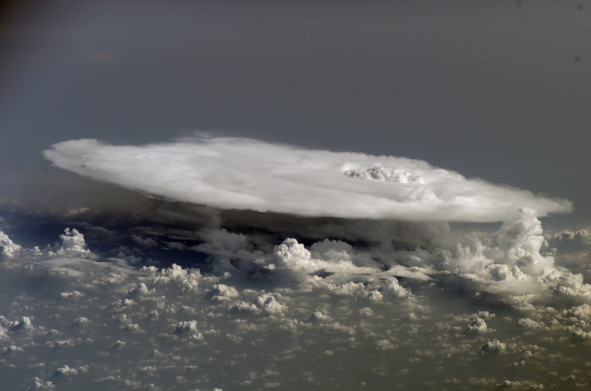
A thunderstorm over Africa, from the ISS. NASA, public domain

Convection: warm air rises 15 km, then spreads under the stratosphere

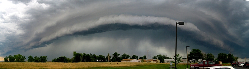
A shelf cloud. NOAA, public domain

A density current: the storm’s cold outflow runs along the ground and lifts the warm air ahead

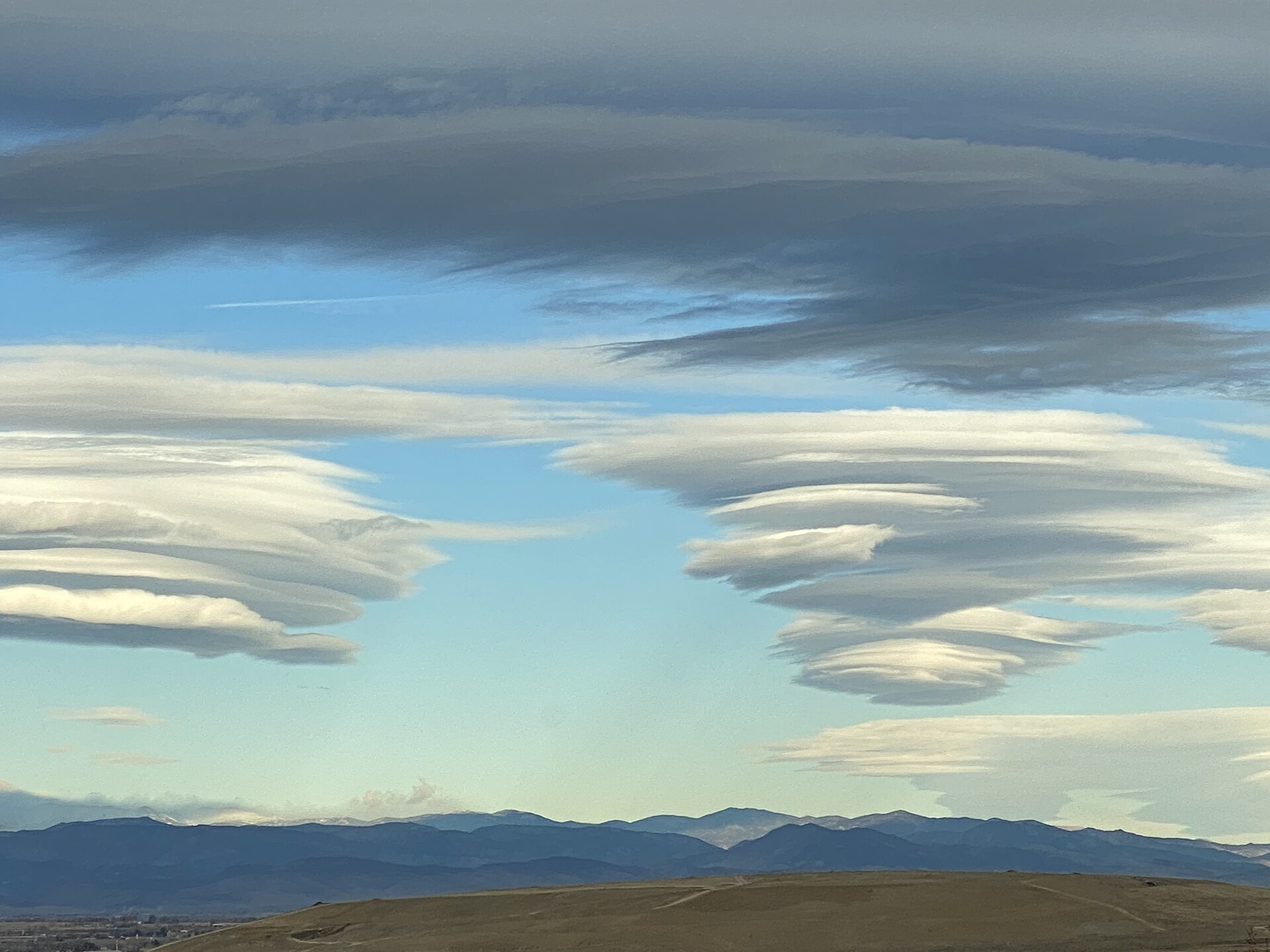
Lenticular clouds, Boulder (Colorado). NOAA, public domain

Mountain waves: air lifted by the Rockies oscillates downstream

Three motions in the vertical, each seen in a vertical plane: what drives them?

Photos: commons: Cumulonimbus cloud over Africa, commons: Shelf cloud 2, commons: Lenticular clouds in Boulder CO

Ask first: why does the anvil stop at about 15 km and spread? (The stratosphere above is very stable.) All three are buoyancy at work; first, how stiff is the layering (next slides).

Layered fluids

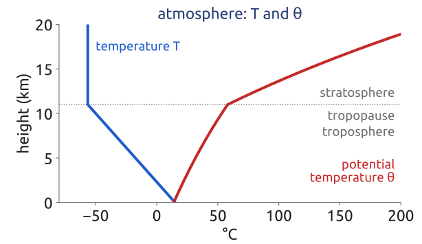
Atmosphere: the temperature falls with height, but the potential temperature \(\theta\) grows: air lifted without heating is colder than its new surroundings

Recall: \(\theta = T\,(p_0/p)^{R/c_p}\) (\(p_0 = 1000\) hPa; \(R\), \(c_p\): of dry air)

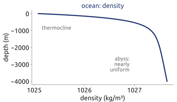
Ocean: light, warm water over dense, cold water; most of the change in a thermocline of a few hundred metres

Both fluids are stably stratified: light over dense

(Vallis 2017; Gill 1982)

Ask first: the temperature falls with height: is the atmosphere then unstable? (No: theta grows.) theta = T (1000 hPa/p)^(R/c_p): the temperature brought down adiabatically to 1000 hPa (lecture 2).

A displaced parcel (1/2): buoyancy pulls it back

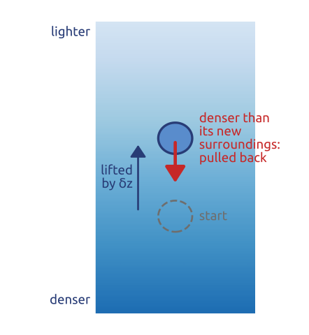
Lift a parcel from \(z_0\) by \(\delta z\); it keeps its density \(\bar\rho(z_0)\). Its new surroundings have \(\bar\rho(z_0 + \delta z) \approx \bar\rho(z_0) + \frac{d\bar\rho}{dz}\delta z\). Its buoyancy, the upward force per unit mass:

\[b = -g\,\frac{\rho_{\mathrm{parcel}} - \rho_{\mathrm{around}}}{\rho_0} = {\color{#1f5ccc}\frac{g}{\rho_0}\frac{d\bar\rho}{dz}}\;\delta z\]

\(\bar\rho(z)\): density of the fluid at rest; \(\rho_0\): constant reference density (Boussinesq)

Density decreasing upwards (\(d\bar\rho/dz < 0\)): \(b < 0\), the parcel is pulled back

A displaced parcel feels the density difference with its new surroundings: its buoyancy

(Vallis 2017; Cushman-Roisin and Beckers 2011)

Boussinesq: rho_0 a constant reference density; density differences matter only through gravity. Ask: pulled back, does the parcel stop at z_0? (No: it arrives with a speed, passes below z_0, is now lighter than its surroundings and is pushed up again: an oscillation, next slide.)

A displaced parcel (2/2): the frequency \(N\)

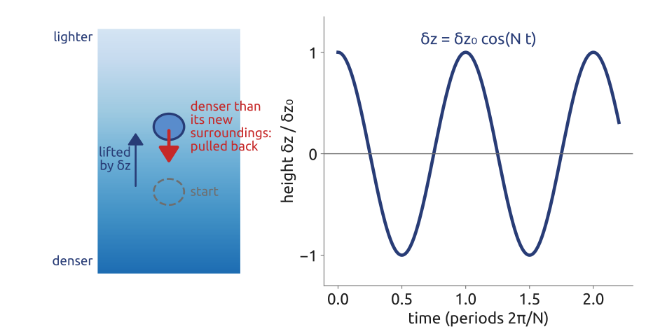
Newton: \(\dfrac{d^2\delta z}{dt^2} = b = -N^2\,\delta z\), with

\[N^2 = -\frac{g}{\rho_0}\frac{d\bar\rho}{dz} \qquad\left(\text{air: } N^2 = \frac{g}{\theta}\frac{d\theta}{dz}\right)\]

\(N\): buoyancy (Brunt–Väisälä) frequency; \(\theta\): potential temperature

\(N^2 > 0\): stable, an oscillation of period \(2\pi/N\), about 10 minutes. \(N^2 < 0\): the parcel runs away: convection

The buoyancy (Brunt–Väisälä) frequency \(N\) measures how stiff the stratification is

(Vallis 2017; Gill 1982)

Ask first: what if the density increased upwards? (Exponential growth, e^{|N| t}: convection.)

Example: how stiff is the stratification?

Each from one gradient (\(g = 9.81\ \mathrm{m\,s^{-2}}\)):

• Summer lake: 24 °C at the top, 12 °C 5 m down, \(N^2 = g\beta_T\,dT/dz\): \(N = 0.069\ \mathrm{s^{-1}}\), 1.5 min
• Troposphere: \(\theta\) grows by 3 K per km at 290 K: \(N = 0.010\ \mathrm{s^{-1}}\), 10 min
• Thermocline: the density grows by 2 kg/m³ over 500 m (\(\rho_0 = 1025\) kg/m³): \(N = 6.2\times10^{-3}\ \mathrm{s^{-1}}\), 17 min
• Abyss: 0.2 kg/m³ over 3000 m: \(N = 8\times10^{-4}\ \mathrm{s^{-1}}\), 2.2 h

\(\beta_T = 2\times10^{-4}\ \mathrm{K^{-1}}\): thermal expansion coefficient, \(\rho = \rho_0[1 - \beta_T(T - T_0)]\)

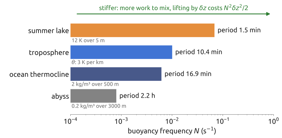
Periods from a minute to hours: the larger \(N\), the more work it takes to mix the water vertically

(Vallis 2017; Gill 1982)

Ask first: which of the four is the hardest to mix vertically? (The lake: lifting a parcel by dz costs N^2 dz^2/2, the integral of N^2 s ds; lake against abyss, N^2 is 7000 times larger.) Lake: N^2 = 9.81 x 2e-4 x 12/5 = 4.7e-3 s^-2: in summer the wind cannot mix its warm top into its cold bottom.

The vertical slice (1/3): the equations

\[\begin{aligned} \frac{D\mathbf{u}}{Dt} + 2\boldsymbol{\Omega}\times\mathbf{u} &= -\frac{1}{\rho_0}\nabla\delta p + b\,\mathbf{k}\\ \nabla\cdot\mathbf{u} &= 0, \qquad \frac{Db}{Dt} = \dot b \end{aligned}\]

\(\delta p\): departure from \(\tilde p(z)\), the hydrostatic pressure of \(\rho_0\) alone; \(b\): buoyancy; \(\dot b\): its sources

In a plane \((x, z)\): \({\color{#1f5ccc}\partial_y = 0,\ v = 0}\); \({\color{#1f5ccc}\boldsymbol{\Omega} = 0}\); \({\color{#1f5ccc}\dot b = 0}\); \({\color{#1f5ccc}\phi = \delta p/\rho_0}\)

\[\begin{aligned} \frac{Du}{Dt} &= -\frac{\partial\phi}{\partial x}, &\quad \frac{Dw}{Dt} &= -\frac{\partial\phi}{\partial z} + b\\[2pt] \frac{Db}{Dt} &= 0, &\quad \frac{\partial u}{\partial x} + \frac{\partial w}{\partial z} &= 0 \end{aligned}\]

\((u, w)\): velocity in the plane; \(D/Dt = \partial_t + u\,\partial_x + w\,\partial_z\)

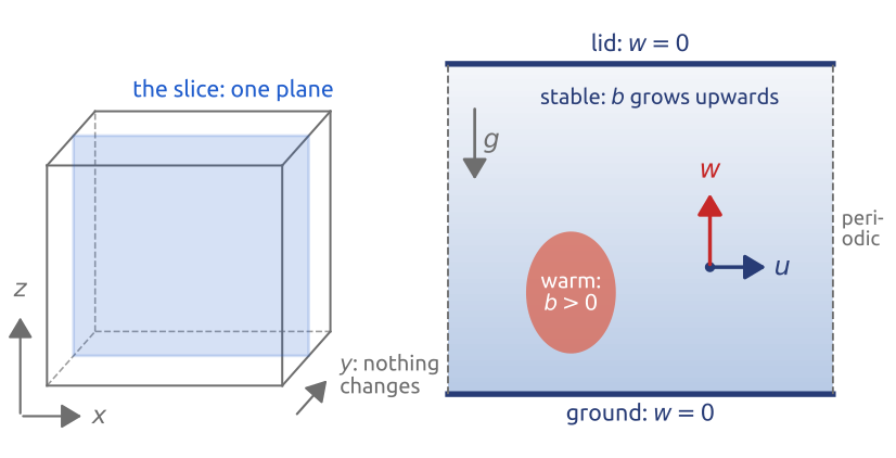
• \(\phi = \delta p/\rho_0\): the pressure departure per unit mass (m²/s²); its gradient is the pressure force
• No rotation: a bubble rises in minutes, \(f\) acts in hours
• Not hydrostatic: \(Dw/Dt\) is kept

But: no equation gives \(\phi\) by itself

The simplest model with up-and-down motion: four equations in a vertical plane

(Vallis 2017; Durran 2010)

Boussinesq: lecture 3. Ask first: which equation of lecture 3 did we drop for shallow water that we keep here? (Dw/Dt.) The pressure is whatever keeps the flow divergence-free: we eliminate it next.

The vertical slice (2/3): buoyancy makes vorticity

1. Vorticity of the slice, positive anticlockwise as drawn: \(\;\xi = \partial_x w - \partial_z u\)
2. \(\partial_x\)(the \(w\) equation) \(-\ \partial_z\)(the \(u\) equation): the pressure drops out \[\partial_x\frac{Dw}{Dt} - \partial_z\frac{Du}{Dt} = \underbrace{-\partial_x\partial_z\phi + \partial_z\partial_x\phi}_{=\,0} + {\color{#1f5ccc}\frac{\partial b}{\partial x}}\]
3. Expand the left side; continuity removes the rest \[\partial_x\frac{Dw}{Dt} - \partial_z\frac{Du}{Dt} = \frac{D\xi}{Dt} + \xi\,\underbrace{\Big(\frac{\partial u}{\partial x} + \frac{\partial w}{\partial z}\Big)}_{=\,0}\]

\[\frac{D\xi}{Dt} = {\color{#1f5ccc}\frac{\partial b}{\partial x}}\]

\(\xi\): minus the \(y\)-component of \(\nabla\times\mathbf u\) (\(y\) points into the page)

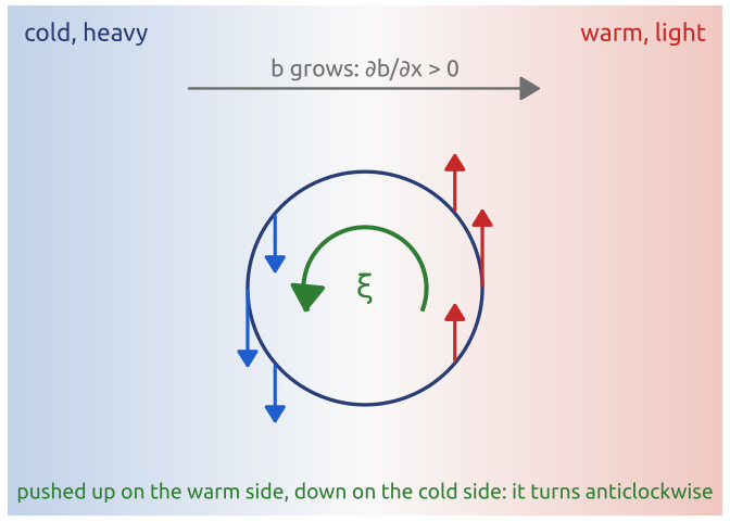
Warm on the right: the fluid turns anticlockwise and rises on the warm side. Bjerknes’s sea breeze (1898) is this equation

But: we now step \(\xi\). Where are \(u\) and \(w\)?

A horizontal buoyancy gradient spins the fluid

(Vallis 2017; Bjerknes 1898)

Sea breeze: lecture 1. Step 3 in full: u_x w_x + w_z w_x - u_x u_z - w_z u_z = xi (u_x + w_z) (notes, line by line). No stretching term: a 2D flow cannot stretch its vortex lines.

The vertical slice (3/3): the 1950 equation

A streamfunction, \(\;u = -\partial_z\psi\), \(\;w = \partial_x\psi\): continuity holds for any \(\psi\), and \(\xi = \nabla^2\psi\). Advection: \(\;\mathbf u\cdot\nabla c = J(\psi, c) = \partial_x\psi\,\partial_z c - \partial_z\psi\,\partial_x c\)

Today, a vertical plane \[\begin{aligned} \partial_t\xi + J(\psi, \xi) &= {\color{#1f5ccc}\partial_x b}\\ \partial_t b + J(\psi, b) &= 0\\ \nabla^2\psi &= \xi \end{aligned}\]

1950, a horizontal plane \[\begin{aligned} \partial_t\zeta + J(\psi, \zeta + f) &= 0\\ \nabla^2\psi &= \zeta \end{aligned}\]

\(\zeta\): vorticity of the horizontal flow; \(f\): Coriolis parameter

Each time step: \(\xi\) and \(b\) forward, then a Poisson problem for \(\psi\), then \(u\) and \(w\)

The vertical slice is the 1950 forecast equation turned on its side, with buoyancy as a source

(Charney et al. 1950; Arakawa 1966)

The 1950 equation: lectures 1 and 3. The notebook codes exactly the left box. Lecture 7 opens the Poisson solver (Fourier).

Internal gravity waves

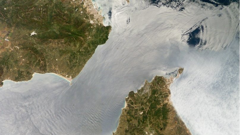
Internal waves leaving the Strait of Gibraltar, from the ISS (cropped). NASA, public domain

In the sea: on the interface between the Atlantic water above and the denser Mediterranean water below; seen from space through the bands of rough and smooth water they make at the surface (sun glint)

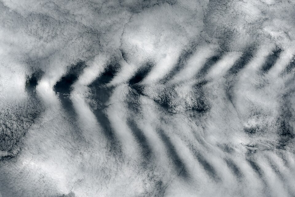
Wave clouds behind Amsterdam Island. NASA Earth Observatory, CC BY 2.0

In the air: behind an island; the air lifted on the wave crests condenses into clouds

But: how fast do they oscillate, and where does their energy go?

Stratified fluids carry waves in their interior: internal gravity waves

(Gill 1982) · Photos: commons: InternalWaves Gibraltar, commons: Wave Clouds behind Amsterdam Island

Ask first: the waves near Gibraltar travel inside the sea, yet they are seen from space: how? (They change the roughness of the sea surface.)

Internal waves (1/2): the dispersion relation

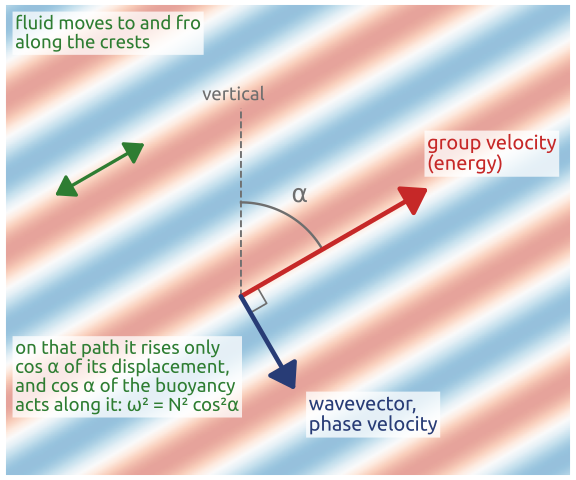
1. Small motions about rest, \(b = N^2 z + b'\): drop the products of small terms in the slice equations; the advection of the background stays, \(J(\psi, N^2 z) = N^2\,\partial_x\psi = N^2 w\) \[\partial_t\xi = \partial_x b', \qquad \partial_t b' = -N^2\,\partial_x\psi, \qquad \xi = \nabla^2\psi\]
2. Take \(\partial_t\) of the first and use the second: \(\;\partial_t^2\,\nabla^2\psi = -N^2\,\partial_x^2\psi\)
3. A plane wave \(\psi \propto e^{i(kx + mz - \omega t)}\): \(\partial_t \to -i\omega\), \(\partial_x \to ik\), \(\partial_z \to im\), so \(\;\omega^2(k^2 + m^2) = N^2 k^2\)

\[\omega^2 = \frac{N^2 k^2}{k^2 + m^2} = N^2\cos^2\alpha, \qquad \omega = N\cos\alpha\]

\(\omega\): frequency; \(k\), \(m\): horizontal and vertical wavenumbers; \(\alpha\): angle of the crests (and of the energy) to the vertical, the same as that of \((k, m)\) to the horizontal: \(\cos\alpha = |k|/\sqrt{k^2 + m^2}\)

Rossby waves: \(\partial_t\nabla^2\psi = -\beta\,\partial_x\psi\) gives \(\omega = -\beta k/(k^2 + l^2)\). The same steps, with \(N^2\) restoring instead of \(\beta\)

The frequency depends on the direction of the wave, not on its length, and never exceeds \(N\)

(Gill 1982; Vallis 2017)

Rossby waves: lecture 3. alpha: angle of the wavevector to the horizontal. The frequency depends on the direction of the wave, not on its length. Vertical crests (alpha = 0, columns moving up and down): omega = N, the parcel.

Internal waves (2/2): energy along the crests

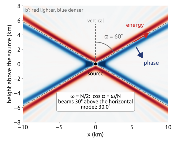
• \(\omega = N\cos\alpha\): every frequency below \(N\) picks one angle; none above \(N\)
• Group velocity \(\partial\omega/\partial\mathbf k\) is perpendicular to \(\mathbf k\): the energy runs along the crests, at the angle \(\alpha\) from the vertical
• A source oscillating at \(\omega < N\) sends four beams: the St Andrew’s cross, an X named after the diagonal cross of St Andrew (Scotland’s flag), first seen in laboratory tanks (Mowbray and Rarity 1967)

Left: the notebook’s slice model, forced at \(\omega = N/2\): beams at \(60^\circ\) from the vertical

Internal waves have frequencies below \(N\), and their energy goes sideways along the crests

(Gill 1982; Vallis 2017; Mowbray and Rarity 1967)

Ask first: shake a source at half the buoyancy frequency: where does the energy go? (Four beams at 60 degrees from the vertical, not in circles.) Phase moves across the beams, energy along them.

Hydrostatic or not?

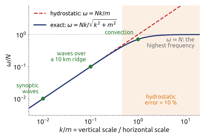
• Hydrostatic balance drops \(Dw/Dt\): then \(\omega = Nk/m\), with no upper limit
• Right when the motion is wide and flat (\(k \ll m\)): weather systems, the large-scale ocean
• Wrong when it is as tall as it is wide: convection, steep mountains, the kilometre scale

Hydrostatic balance holds for wide motions; kilometre-scale models must be non-hydrostatic

(Durran 2010; Vallis 2017)

Hydrostatic balance: lecture 3. Ratio of the two frequencies: sqrt(1 + k^2/m2): 10 % at k/m = 0.46. Lecture 9: km-scale models.

Convection (1/2): a warm bubble, a vortex pair

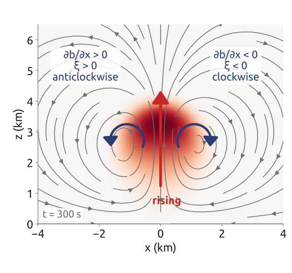
• Inside the bubble’s centre \(\partial_x b = 0\); on its flanks it is not
• Left flank, \(\partial_x b > 0\): \(D\xi/Dt > 0\), anticlockwise. Right flank: clockwise
• The two vortices lift the air between them and bring it down outside: in 3D, a vortex ring, as a smoke ring

Left: the notebook’s bubble after 5 minutes, with its streamlines

But: what shape does it take, and how fast does it rise?

A warm bubble does not rise as a ball: its flanks spin up a vortex pair

(Robert 1993; Bryan and Fritsch 2002)

Ask first: drop a ball of warm air: will it rise as a ball? (No: a vortex pair; a mushroom, as a smoke ring or the cloud of an explosion.)

Convection (2/2): a mushroom

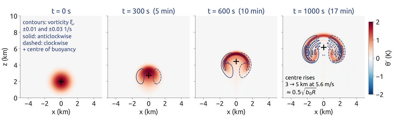
• Bryan and Fritsch’s dry bubble: \(\theta' = 2\) K warmer than \(\theta_0 = 300\) K, radius \(R = 2\) km. Scale: \(\sqrt{bR} \approx 11\) m/s, with \(b = g\theta'/\theta_0\); the centre rises at about half of it (5.6 m/s), the core at 16 m/s
• The cap rolls up into a mushroom

But: a cold bubble falls. What does it do at the ground?

Buoyancy accelerates, the vortex pair shapes: rise speeds of order \(\sqrt{bR}\)

(Bryan and Fritsch 2002; Robert 1993)

b = 9.81*2/300 = 0.065 m/s^2, sqrt(bR) = 11 m/s. Notebook 4a, 100 m grid, nu = 20 m^2/s. The small negative theta’ at the edges: ripples of the centred scheme (lecture 5).

A cold bubble: a density current

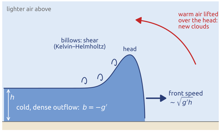
A shelf cloud on a gust front. NOAA, public domain

• Cold air reaches the ground and spreads as a density current, at about \(\sqrt{g'h}\) (\(h\): its depth; \(g' = g\,|\theta'|/\theta_0\): reduced gravity)
• Thunderstorm gust fronts; sea-breeze fronts; dense Mediterranean water leaving Gibraltar along the bottom
• Straka et al. (1993): a \(-15\) K bubble, the benchmark of every non-hydrostatic model

Heavy fluid runs under light fluid, with a head and billows: the same picture in air and in water

(Straka et al. 1993; Benjamin 1968) · Photo: commons: Shelf cloud 2

Sea breeze: lecture 1. g’ = g |theta’|/theta_0. Straka: front speed over 30 m/s at 300 s, about 15 m/s at 900 s; the billows (Kelvin-Helmholtz) need viscosity (75 m^2/s) for a converged reference solution.

Notebook The vertical slice

Notebook 04a (open in Colab · download): the vertical slice on a computer, three equations and a Poisson problem.

The model: one vertical plane, periodic sides, lids at the ground and the top

1. The equations and the model: a standing wave checks \(\omega = N\cos\alpha\)
2. A warm bubble: the vortex pair, the mushroom, a rise speed of order \(\sqrt{bR}\)
3. A cold bubble: Straka’s density current, its front against \(\sqrt{g'h}\)
4. An oscillating source: the St Andrew’s cross ❗ 4.1
5. An unstable layer: convective cells grow from noise ❗ 5.1

Predict, run, explain: write down what you expect before each run

One model, three equations: bubbles, density currents and internal waves on a computer

(Bryan and Fritsch 2002; Straka et al. 1993; Mowbray and Rarity 1967)

In class, 25 min: sections 2 and 4 (with exercise 4.1); sections 1, 3 and 5 (with exercise 5.1) at home. The model is a black box today; its numerics come in the second week. If time is short: section 4 only. Exercise 4.1: 0.3N: beams 17.5 degrees above the horizontal (72.5 from the vertical); 0.8N: 53.1 (36.9); above N no waves, the response stays at the source. Model: 17.3, 30.0, 53.3.

What the notebook showed

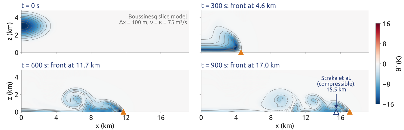
• Front at 900 s: 17.0 km on this 100 m grid (16.7 km at 200 m), converging to 16.8 km on finer grids; Straka’s compressible reference: 15.5 km. The Boussinesq version runs 8 % ahead: the equations, not the grid
• Front speed 16 m/s, about \(1.4\sqrt{g'h}\); the billows need \(\nu = 75\ \mathrm{m^2/s}\) to converge

Converged solutions need resolved (or fixed) dissipation

(Straka et al. 1993)

Fronts at 900 s: 16.3, 16.7, 17.0, 16.9, 16.8 km at 400, 200, 100, 50, 25 m. Without viscosity the run stays bounded but theta’ overshoots to +11 K: no converged solution.

Convection in coarse models

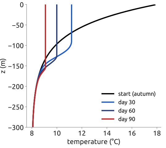
A column model: winter cooling deepens the ocean’s mixed layer (optional notebook)

• A thunderstorm’s updraft is 1–10 km wide: a global model with 9 km cells cannot see it
• Instead, each column is checked: where \(N^2 < 0\), a parameterization mixes it (the simplest: convective adjustment)
• Between about 10 and 1 km, deep convection is partly resolved: the grey zone (partly resolved, partly parameterized)
• The ocean convects too, in winter: the Gulf of Lion, the Labrador and Greenland Seas

What a fine model resolves, a coarse one must parameterize, column by column

(Marshall and Schott 1999; Durran 2010)

Grey zone: lecture 9. The column notebook (extra block) implements convective adjustment with an implicit vertical step.

Air forced up by a mountain

Lenticular clouds over the Rocky Mountains. NOAA, public domain

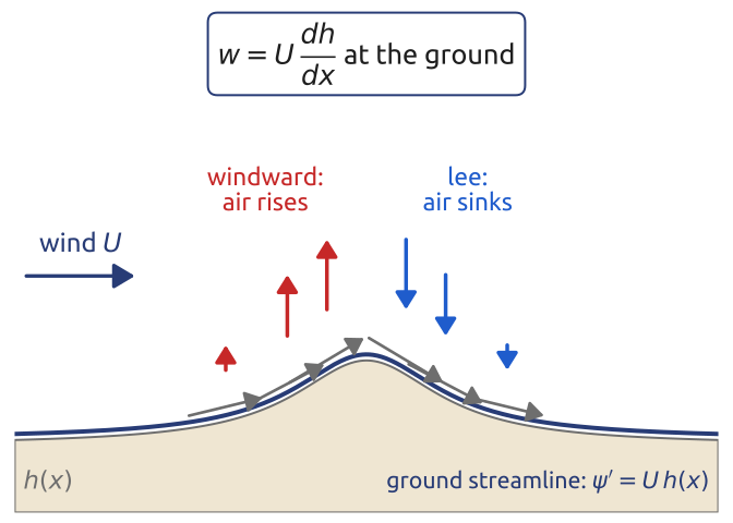
A wind \(U\) over the ground \(z = h(x)\). The ground is a streamline: \(w = U\,dh/dx\) there

But: does the push stay near the ground, or reach the stratosphere?

A mountain forces vertical motion: in a stratified fluid, that makes waves

(Queney 1948; Smith 1979) · Photo: commons: Lenticular clouds in Boulder CO

Ask first: do the waves tilt with the wind or against it? (Against: upstream.)

Mountain waves (1/2): linear theory

Steady flow, \(\partial_t \to 0\), \(\;\mathbf u\cdot\nabla \to U\partial_x\); the slice equations give

\[\nabla^2\psi' + \frac{N^2}{U^2}\,\psi' = 0, \qquad \psi'(x, 0) = U\,h(x)\]

\(\psi'\): streamfunction of the disturbance, \(\psi = -Uz + \psi'\); \(U\): uniform wind; \(h(x)\): height of the ground

Fourier in \(x\): \(\hat\psi(k, z) = U\hat h(k)\,e^{imz}\), \(\;m^2 = \dfrac{N^2}{U^2} - k^2\)

\(\hat{\ }\): Fourier transform in \(x\); \(k\), \(m\): horizontal and vertical wavenumbers

• \(|k| < N/U\) (wide mountains): \(m\) real, waves go up, tilting upstream
• \(|k| > N/U\) (narrow): \(m\) imaginary, the disturbance decays with height

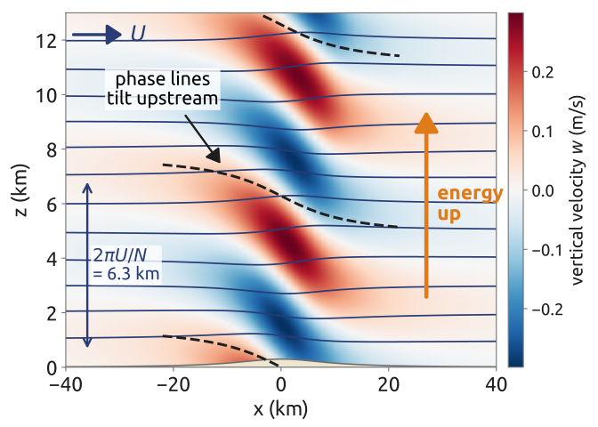
The mountain’s width against \(U/N\) decides: waves aloft, or a disturbance that fades

(Queney 1948; Durran 1990)

U/N = 1 km for 10 m/s and 0.01 1/s. The sign of m: energy must go up (radiation condition), which makes the phase lines tilt upstream. Queney (1948) solved the hydrostatic case in closed form.

Mountain waves (2/2): three regimes

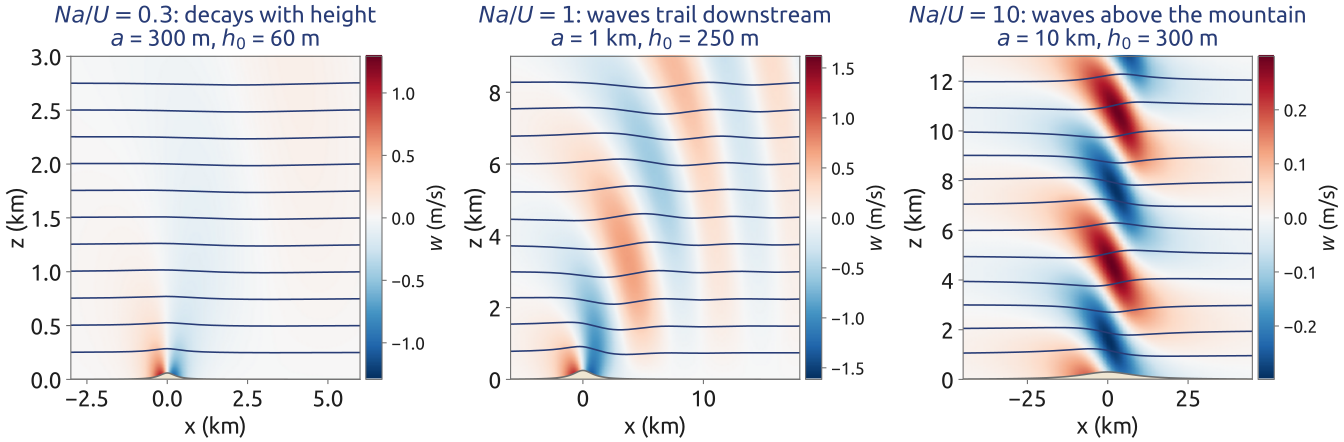
\(Na/U \ll 1\): decays, no waves aloft · \(Na/U \approx 1\): non-hydrostatic waves trailing downstream · \(Na/U \gg 1\): hydrostatic waves above the mountain, vertical wavelength \(2\pi U/N \approx 6\) km

One number, \(Na/U\), sorts the flow over a mountain of half-width \(a\)

(Queney 1948; Smith 1979)

Ask first: which mountain makes waves that reach the stratosphere, the narrow or the wide one? (Wide.)

Lee waves and wave clouds

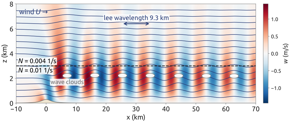
The Scorer parameter (Scorer 1949), \(\;l^2(z) = \dfrac{N^2}{U^2} - \dfrac{U''}{U}\) (\(U''\): curvature \(d^2U/dz^2\) of the wind profile; constant \(U\): \(l = N/U\))

Wave clouds behind Amsterdam Island. NASA Earth Observatory, CC BY 2.0

When \(l\) falls with height, waves cannot go up: they are trapped and trail far downstream

Trapped lee waves: wave trains downstream, with clouds on their crests

(Scorer 1949; Durran 1990) · Photo: commons: Wave Clouds behind Amsterdam Island

Scorer parameter l, l^2(z) = N^2/U2 - U’’/U (l = N/U for constant U). Lee wavelengths between 2 pi/l_lower and 2 pi/l_upper, typically 5-20 km.

High mountains: blocking and downslope winds

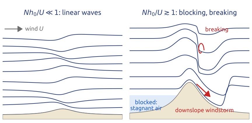
• A mountain of height \(h_0\): can the air climb it? Lifting it by \(h_0\) costs about \(N^2h_0^2/2\); it has \(U^2/2\)
• \(Nh_0/U \ll 1\): linear waves. \(Nh_0/U \gtrsim 1\): the low air is blocked; aloft the waves steepen and break
• Downslope windstorms (bora, foehn); an isolated mountain, as the Alps, makes the low air go around it

A second number, \(Nh_0/U\), says when linear theory stops: blocking and breaking

(Durran 1990; Smith 1979)

2D: upstream blocking for Nh/U above about 1; 3D: flow splitting around isolated mountains. The Po valley’s winter fog: cold air blocked by the Alps and the Apennines (next slide).

Example: waves or blocking?

\(N = 0.01\ \mathrm{s^{-1}}\), \(U = 10\) m/s: \(U/N = 1\) km, vertical wavelength \(2\pi U/N = 6.3\) km

• A hill, \(a = 500\) m, \(h_0 = 50\) m: \(Na/U = 0.5\), \(Nh_0/U = 0.05\): flows over, no waves aloft
• A ridge, 10 km, 500 m: 10 and 0.5: hydrostatic waves above it, tilting upstream
• The Alps, 100 km, 3 km: 100 and 3: blocked; the low air goes around
• The Apennines, 20 km, 1.2 km. Winter inversion, \(N = 0.03\ \mathrm{s^{-1}}\), \(U = 2\) m/s: 300 and 18, blocked: the Po valley keeps its cold air, its fog and its smog. Summer afternoon, \(N = 0.005\ \mathrm{s^{-1}}\), \(U = 10\) m/s: 10 and 0.6, the air flows over and makes waves

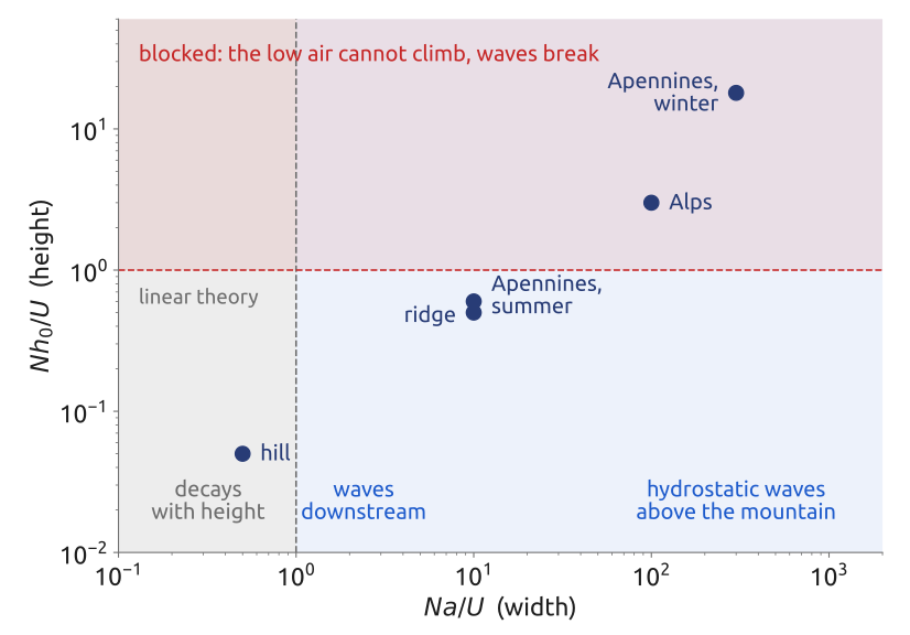
Two numbers place any mountain: a winter inversion turns the Apennines into a wall

(Smith 1979; Durran 1990)

Ask first: the same Apennines in winter and in summer: which one blocks the air? (Winter: strong N, weak wind.) The Alps are wide enough for rotation too: U/(fa) = 1.

Notebook Mountain waves

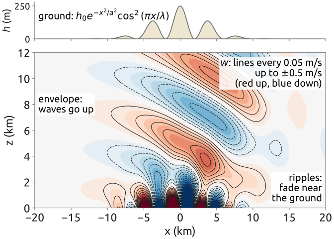
Notebook 04b (open in Colab · download) (demo, or at home):

1. Linear theory by FFT, checked against Queney’s (1948) solution
2. The three regimes; the drag on the mountain ❗ 2.1 (your own mountain)
3. Trapped lee waves
4. Schär’s mountain (left): short ripples fade, the long envelope makes waves
5. A time-dependent model: what the top of the domain must do ❗ 5.1

Linear theory gives exact answers to check models against

(Queney 1948; Schär et al. 2002)

Exercises 2.1 (your own mountain: Na/U, Nh0/U, the linear solution, where it overturns) and 5.1 (the depth and strength of the sponge) are mandatory. Section 5: the sponge layer at the top of a model (lecture 9).

Key points

1. Stratification: \(N^2 = -(g/\rho_0)\,d\bar\rho/dz\), periods of minutes; \(N^2 < 0\): convection
2. The slice: \(D\xi/Dt = \partial_x b\), \(\;\nabla^2\psi = \xi\): buoyancy gradients make vorticity; a Poisson problem each step
3. Internal waves: \(\omega = N\cos\alpha < N\), energy along the crests; hydrostatic fails for motions as tall as wide
4. Convection: warm bubbles rise as vortex pairs; cold air spreads as a density current at about \(\sqrt{g'h}\)
5. Mountains: \(Na/U\) (waves or decay), \(Nh_0/U\) (blocking); waves tilt upstream, wavelength \(2\pi U/N\)

Notebook 04a (open in Colab · download): the bubbles, the density current and the waves of today; notebook 04b (open in Colab · download): the mountain waves; optional: 04c (open in Colab · download), the vertical modes, and 04d (open in Colab · download), mixing in a column.

The vertical slice: the 1950 vorticity equation on its side, driven by buoyancy

Reading: (Vallis 2017; Gill 1982, Ch. 6 and 8; Durran 1990, 2010)

Lecture 7’s warm-up asks about the slice. The vertical modes (the slides after this one) are optional. Next: the numerics, from the start: grids, time steps and the CFL condition (lecture 5). The Poisson solve of every step: Fourier and spherical harmonics (lecture 7); the vertical in real models: lecture 9.

Extra: vertical modes (optional)

How a layered fluid splits into a stack of shallow water systems, each with its own wave speed and deformation radius. For self-study; models with semi-implicit time steps use these modes.

(Gill 1982, sec. 6.11; Vallis 2017, sec. 3.4.1)

The semi-implicit method of lecture 7 uses these modes.

Vertical modes (1/3): the linear equations

Small motions about rest; hydrostatic, Boussinesq, \(f\)-plane, rigid lid, flat bottom:

\[\begin{aligned} &\partial_t u - f v = -\partial_x \phi, \qquad \partial_t v + f u = -\partial_y \phi\\ &{\color{#1f5ccc}\partial_z \phi = b}, \qquad {\color{#1f5ccc}\partial_t b + N^2(z)\, w = 0}\\ &\partial_x u + \partial_y v + \partial_z w = 0, \qquad w = 0 \text{ at } z = -H, 0 \end{aligned}\]

\(\phi = \delta p/\rho_0\): pressure departure per unit reference density; \(b\): buoyancy, departure from the mean \(\bar b(z)\), with \(N^2 = d\bar b/dz\). In blue: what is new since shallow water

Hydrostatic \(\partial_z p = -\rho g\) becomes \(\partial_z\phi = b\) for the perturbations; Boussinesq: \(\rho_0\) everywhere except in \(b = -g(\rho - \rho_0)/\rho_0\)

(Gill 1982; Vallis 2017)

Hydrostatic: the vertical momentum equation reduced to dp/dz = -rho g (lecture 3). The buoyancy equation: b changes only by vertical motion across the mean stratification.

Vertical modes (2/3): separate the variables

Look for \(\;(u, v, \phi) = (\hat u, \hat v, \hat\phi)(x, y, t)\;{\color{#1f5ccc}C(z)}\), \(\;w = \hat w(x, y, t)\;{\color{#1f5ccc}W(z)}\), with \(C = dW/dz\)

• continuity: \(\hat w = -(\partial_x\hat u + \partial_y\hat v)\)
• hydrostatic + buoyancy: \(\partial_t\hat\phi\; C' + N^2\, \hat w\, W = 0\)
• divide: \(z\) on one side, \((x, y, t)\) on the other: both \(= -1/c^2\)

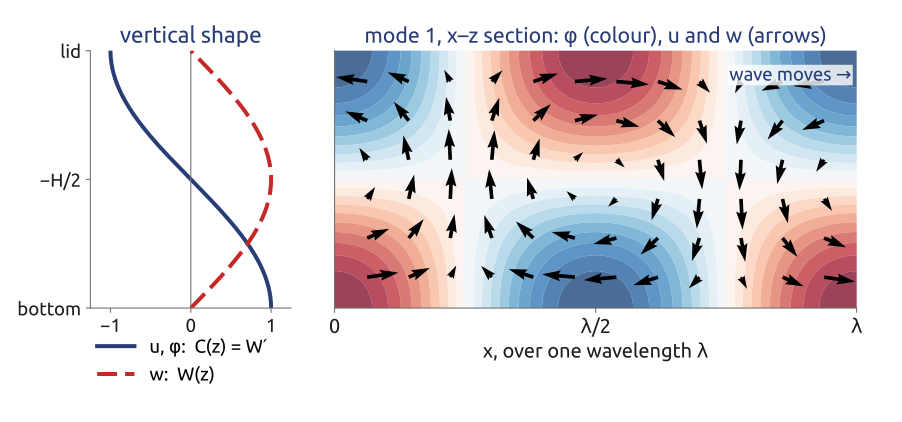
Every field is a horizontal pattern times a fixed vertical shape

(Gill 1982, sec. 6.11; Vallis 2017, sec. 3.4.1)

The same trick as for the heat equation or the vibrating string. C gives the shape of the horizontal velocity and of the pressure (Vallis’s C_m, 3.4.1; W is Gill’s R, 6.11).

Vertical modes (3/3): shallow water per mode

Vertical: a Sturm–Liouville problem

\[W'' + \frac{N^2(z)}{c^2}\,W = 0,\qquad W(-H) = W(0) = 0\]

Eigenvalues \(c_1 > c_2 > \dots\) (mode index \(m\), not a wavenumber); constant \(N\): \(c_m = NH/(m\pi)\). Equivalently \(C = dW/dz\) obeys \((C'/N^2)' + C/c^2 = 0\)

Horizontal: linear shallow water

\[\partial_t\hat\phi + {\color{#1f5ccc}c^2}\,(\partial_x\hat u + \partial_y\hat v) = 0\]

with \(gH \to c_m^2\): an equivalent depth \(H_m = c_m^2/g\), a deformation radius \(L_m = c_m/f\) (below: \(H_m\), \(c_m\), \(L_m\) at Milan)

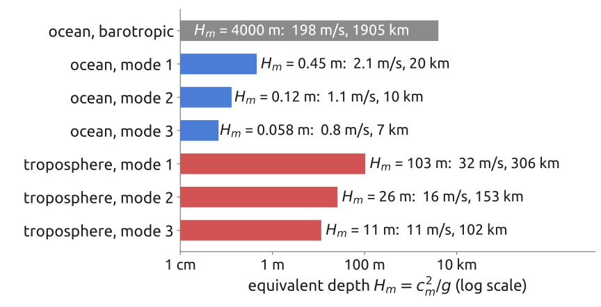
A stratified fluid is a stack of shallow water systems, one per vertical mode

(Gill 1982, sec. 6.11; Vallis 2017, sec. 3.4.1)

Shallow water: lecture 3. Ask first: which mode has the largest speed? (The first: one zero crossing.) With a free surface there is also the barotropic mode, c_0 = sqrt(gH): 200 m/s in a 4 km ocean.

The modes of the ocean

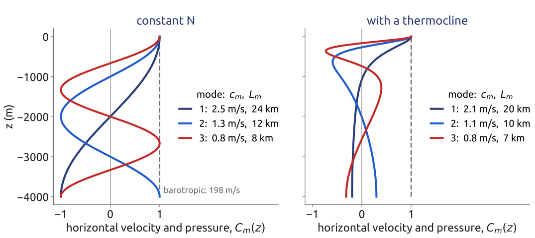
First baroclinic mode: 2 m/s, \(L_1 \approx 20\) km at Milan: the size of ocean eddies. The barotropic mode: 200 m/s, 1900 km. The atmosphere: \(c_1 = NH/\pi \approx 30\) m/s, \(L_1 = c_1/f \approx 300\) km (the deformation radius \(L_d = NH/f \approx 1000\) km is \(\pi\) times larger).

The ocean’s eddies are ten times smaller than the atmosphere’s cyclones: a deformation radius

(Gill 1982, sec. 6.11; Vallis 2017, sec. 3.4.1)

This is why global ocean models need grids of a few km to resolve eddies (lecture 6, L_d/dx). Left: constant N, exact cosines. Right: the thermocline squeezes the modes towards the surface.

Example: how fine must an ocean model be?

Constant \(N\): \(c_1 = NH/\pi\), \(H_1 = c_1^2/g\), \(L_1 = c_1/f\), at Milan (\(f = 1.04\times10^{-4}\ \mathrm{s^{-1}}\)):

• Ocean, \(N = 2\times10^{-3}\ \mathrm{s^{-1}}\), \(H = 4\) km: \(c_1 = 2.5\) m/s, \(H_1 = 0.66\) m, \(L_1 = 24\) km
• Troposphere, \(N = 10^{-2}\ \mathrm{s^{-1}}\), \(H = 10\) km: 32 m/s, 103 m, 306 km
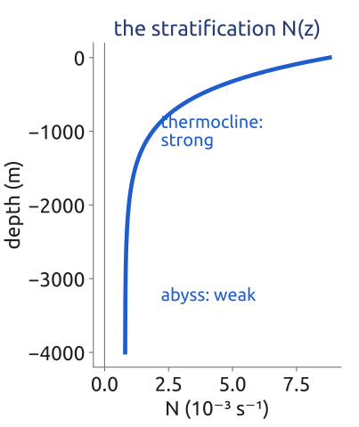
• Ocean with a thermocline, \(N(z)\) of the slides before: \(c_1 \approx \frac{1}{\pi}\int_{-H}^{0} N\,dz = 2.3\) m/s (the eigenvalue solver: 2.1 m/s)
• To see eddies a grid needs \(\Delta x \lesssim L_1/3\): 15 km at \(20^\circ\)N, 7 km at Milan, 6 km at \(70^\circ\)N

\(\int N\,dz/(m\pi)\): the WKB estimate of \(c_m\)

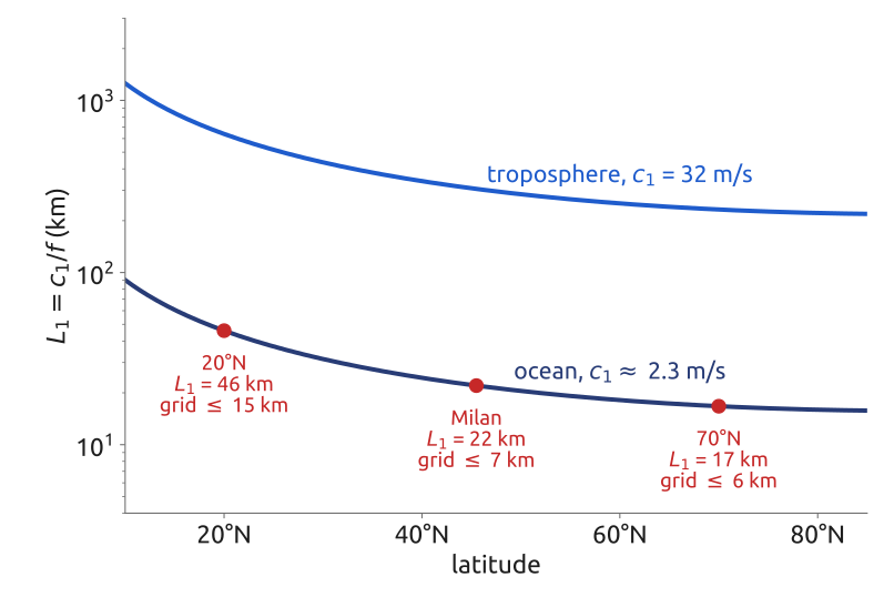
An ocean model needs a grid of a few kilometres to see its eddies, finer towards the poles

(Gill 1982, sec. 6.11; Vallis 2017, sec. 3.4.1)

Integral of N: 8e-3 x 500 + 8e-4 x 4000 = 4.0 + 3.2 = 7.2 m/s, c_1 = 2.29 m/s. L_1/3 is a rule of thumb (two to three points per radius). Eddy-resolving global ocean models: about 1/10 degree.

Notebook Vertical modes

The input: \(N(z)\) of the notebook’s ocean

Open notebook 04c (open in Colab · download) (optional, 25 min):

1. A stratified ocean: density and \(N(z)\)
2. The mode problem as a matrix eigenvalue problem (finite differences)
3. Check against constant \(N\): which order of accuracy?
4. The modes of an ocean with a thermocline: speeds, equivalent depths, deformation radii

Predict first: where will mode 1 have its strongest currents?

A Sturm–Liouville problem becomes scipy.linalg.eigh(A, B)

(Gill 1982)

Finite differences: lecture 5. Error falls by 4 when the grid is halved: second order. WKB estimate c_m = (1/(m pi)) integral N dz.

Notebook A column model of the mixed layer

Open notebook 04d (open in Colab · download) (optional, 20 min):

1. Vertical diffusion, explicit: the step limit \(\Delta z^2/2K\)
2. Implicit (backward Euler): one tridiagonal solve per step of 1 hour
3. A winter of cooling: convective adjustment deepens the mixed layer

Predict first: how deep is the mixed layer after 90 days of losing 200 W/m²?

Column physics: what models add, column by column, to the resolved dynamics

(Durran 2010; Griffies et al. 2000)

Heat is conserved to round-off (finite volumes). Notebook exercise 3: Crank–Nicolson oscillates for stiff modes, backward Euler damps them.