Finite differences: time stepping, advection and the CFL condition
Atmosphere and Ocean Dynamics, Lecture 5: notes
Finite differences: how a grid model turns the equations into numbers stepped forward in time. These notes discuss the method of lines and the order of difference formulas; normal modes, the amplification factor and the stability of forward and backward Euler, the trapezoidal scheme, leapfrog with the Robert–Asselin filter and Runge–Kutta schemes; von Neumann’s analysis of advection schemes, the CFL condition and the Lax–Richtmyer theorem; numerical diffusion and dispersion; gravity waves on the A and C grids; and the Courant numbers of Richardson’s forecast and of the ENIAC’s.
1 Warm-up
The questions recall the equations whose numerics this lecture builds.
- A tracer \(q\) carried by a constant wind \(c\). \(\partial_t q + c\,\partial_x q = 0\), with the exact solution \(q(x, t) = q_0(x - ct)\): the initial shape moves unchanged at the speed \(c\).
- The inertial oscillation \(du/dt = fv\), \(dv/dt = -fu\). With \(w = u + iv\), \(dw/dt = -ifw\), so \(w = w_0\,e^{-ift}\): \(|w|\) stays constant and the velocity turns clockwise, once in \(2\pi/f\) (16.8 h at Milan, \(f = 1.04\times10^{-4}\ \mathrm{s^{-1}}\)).
- Linear shallow water in one dimension, with rotation. \(\partial_t\eta + H\,\partial_x u = 0\), \(\partial_t u - fv = -g\,\partial_x\eta\), \(\partial_t v + fu = 0\), for a layer of mean depth \(H\) with surface elevation \(\eta\).
- Wave speeds. Gravity waves travel at \(\sqrt{gH}\): 198 m/s in an ocean 4000 m deep, 280 m/s for an atmosphere with \(H \approx 8\) km. The first baroclinic mode of the ocean, \(c_1 = NH/\pi\) with \(N = 2\times10^{-3}\ \mathrm{s^{-1}}\), travels at 2.5 m/s. The fastest wave will set the time step of explicit schemes.
- What else the 1950 forecast and the vertical slice solve at every step. A Poisson problem, \(\nabla^2\psi = \zeta\), for the streamfunction \(\psi\) of the vorticity \(\zeta\) being stepped forward.
2 Richardson (1922): the method, and a time step
Richardson (1922) computed by hand, for 07 UTC on 20 May 1910, the tendencies of the primitive equations at two points over central Europe, and found a surface pressure change of 145 hPa in six hours, against an almost steady barometer. The main reason is the initial state: the observed winds and pressures were out of balance, and the imbalance projects on fast gravity waves; with the data filtered, Lynch’s reconstruction gives a realistic tendency (Lynch 1999, 2008).
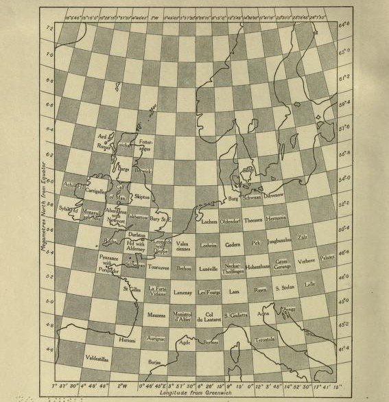
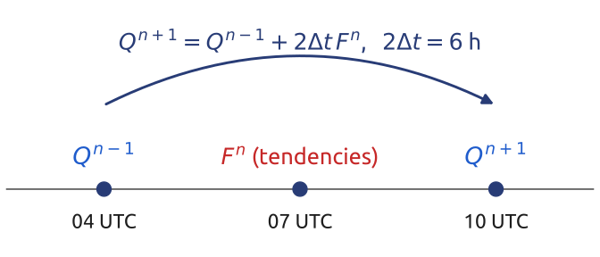
The slide looks at the other half of the problem, the time step. Richardson’s grid had points every \(3^\circ\) of longitude and \(1.8^\circ\) of latitude, about 200 km, on a staggered chequer-board now called the E grid (Figure 1). His time scheme was what he called the step-over method and we call leapfrog: the tendency \(F^n\) at 07 UTC moves the state from 04 UTC to 10 UTC (Figure 2), \[ Q^{n+1} = Q^{n-1} + 2\Delta t\,F^n, \qquad 2\Delta t = 6\ \mathrm{h}. \] As Lynch (1999) points out, the time step is then \(\Delta t = 3\) h, “not six hours as so often stated”. Had his data been balanced, could he have gone on, step after step, to a 24-hour forecast? This lecture shows that he could not (Section 34).
3 The method of lines: space first, then time
A model of the atmosphere or the ocean is a set of partial differential equations, \(\partial_t q = \mathcal F(q)\), where \(\mathcal F\) contains the space derivatives. Most models discretize them in two separate steps (Durran 2010, sec. 1.3):
- Space. Keep the values \(q_j(t) \approx q(x_j, t)\) at grid points \(x_j = j\,\Delta x\) and replace the space derivatives by differences of neighbouring values. For the advection equation with the centred difference, \[ \frac{dq_j}{dt} = -c\,\frac{q_{j+1} - q_{j-1}}{2\Delta x}. \]
- Each \(q_j\) now obeys an ordinary differential equation; together they form one large system, \[ \frac{d\mathbf q}{dt} = \mathbf F(\mathbf q), \] with \(\mathbf q\) the vector of all grid values and \(\mathbf F\) their tendencies.
- Time. Advance this system with a time step \(\Delta t\): \(q_j^n \approx q(x_j, t^n)\), \(t^n = n\,\Delta t\).
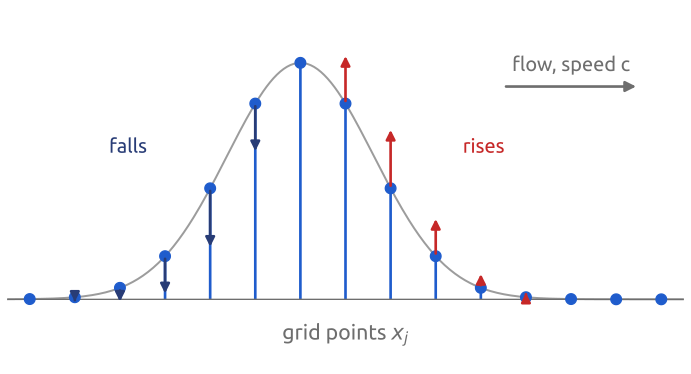
This is the method of lines: each grid value moves along its own line in time (Figure 3). Finite volumes, spectral methods and finite elements replace the first step by fluxes between cells or by expansions in functions, but keep the second. Two questions follow for every scheme: how accurate is a difference, and does a time step keep the errors bounded?
4 Taylor series (1/3): a derivative from grid values
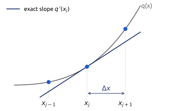
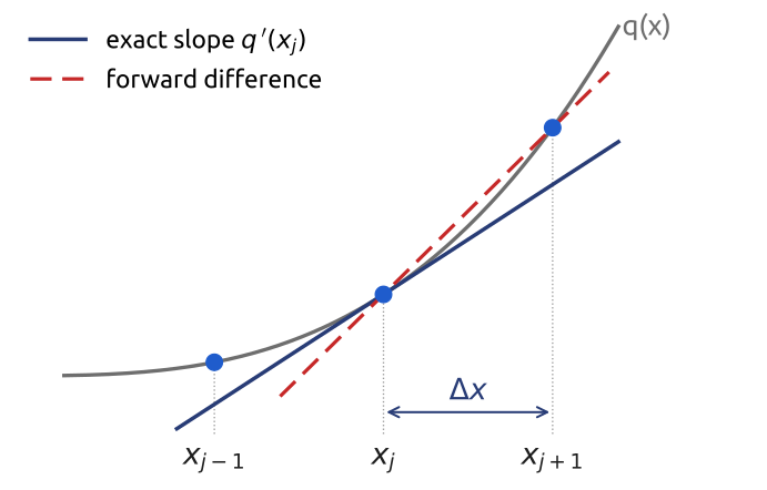
On a grid only values are known; derivatives must be built from them. Let \(q\) be smooth, and expand it about \(x_j\) one grid step ahead and one behind (Durran 2010, sec. 1.3.1, §3.1): \[ \begin{aligned} q_{j+1} &= q_j + \Delta x\,q'_j + \frac{\Delta x^2}{2}\,q''_j + \frac{\Delta x^3}{6}\,q'''_j + O(\Delta x^4),\\ q_{j-1} &= q_j - \Delta x\,q'_j + \frac{\Delta x^2}{2}\,q''_j - \frac{\Delta x^3}{6}\,q'''_j + O(\Delta x^4). \end{aligned} \tag{1}\] The question is which combination of \(q_{j-1}\), \(q_j\) and \(q_{j+1}\) gives \(q'_j\) best (Figure 4).
5 Taylor series (2/3): forward difference
Solving the first line of Equation 1 for \(q'_j\) gives the forward difference, \[ \frac{q_{j+1} - q_j}{\Delta x} = q'_j + \frac{\Delta x}{2}\,q''_j + O(\Delta x^2). \] The terms left over are the truncation error: what the difference leaves out of the Taylor series. A difference is of order \(p\) if its truncation error falls like \(\Delta x^p\); the forward difference, and the backward one, \((q_j - q_{j-1})/\Delta x\), are first order: halving \(\Delta x\) halves the error [Durran (2010), §3.1; §3.3.2, eq. 3.39]. Geometrically, the forward difference is the slope of the secant through \(x_j\) and \(x_{j+1}\) (Figure 5).
6 Taylor series (3/3): centred is second order
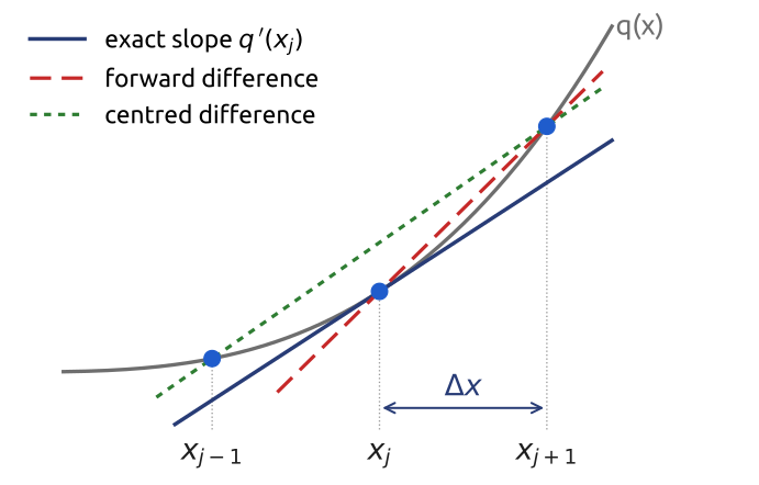
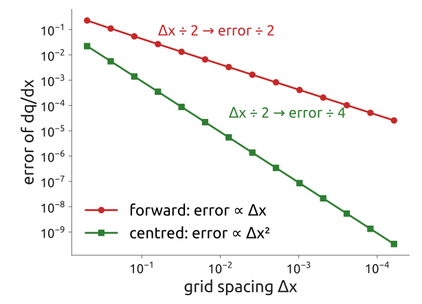
Subtracting the second line of Equation 1 from the first, the even powers of \(\Delta x\) cancel, and the centred difference is second order: \[ \frac{q_{j+1} - q_{j-1}}{2\Delta x} = q'_j + \frac{\Delta x^2}{6}\,q'''_j + O(\Delta x^4). \] Its secant, through \(x_{j-1}\) and \(x_{j+1}\), is almost parallel to the tangent (Figure 6). The order is checked on a log–log plot of the error against \(\Delta x\): halving \(\Delta x\) must divide the error by \(2^p\) (Figure 7, for \(q = \sin x\) at \(x = 1\); the ratios are 2.0 and 4.0). This is a test for any code. With more points one can cancel more terms (the fourth-order centred difference uses \(q_{j\pm1}\) and \(q_{j\pm2}\)). But accuracy at one instant is not enough: the errors must also not grow when the solution is stepped in time.
7 Normal modes: one equation for all waves
A time scheme is judged on one ordinary differential equation, because every linear wave reduces to it. Take the linear gravity waves in one dimension without rotation, \[ \partial_t\eta + H\,\partial_x u = 0, \qquad \partial_t u + g\,\partial_x\eta = 0 . \] One Fourier mode, \((\eta, u) = (\hat\eta, \hat u)\,e^{ikx}\), turns them into a linear system of two ordinary differential equations, \[ \frac{d}{dt}\begin{pmatrix}\hat\eta\\ \hat u\end{pmatrix} = \mathsf M\begin{pmatrix}\hat\eta\\ \hat u\end{pmatrix}, \qquad \mathsf M = \begin{pmatrix}0 & -iHk\\ -igk & 0\end{pmatrix}. \] Its eigenvalues solve \(\det(\mathsf M - \lambda\mathsf I) = \lambda^2 + gHk^2 = 0\), so \(\lambda = \pm ick\) with \(c = \sqrt{gH}\). From the first row, \(-iHk\,\hat u = \lambda\hat\eta\): the eigenvectors are \((\hat\eta, \hat u) = (H, \mp c)\). The mode with \(\lambda = +ick\) varies as \(e^{ik(x + ct)}\), a wave going left with \(u = -c\eta/H\); the one with \(\lambda = -ick\) goes right, with \(u = +c\eta/H\).
In the basis of the eigenvectors, \(\mathsf M = \mathsf Q\mathsf\Lambda\mathsf Q^{-1}\) with \(\mathsf\Lambda\) diagonal, the system splits into independent scalar equations, one per wave: the oscillation equation \[ \frac{d\psi}{dt} = \lambda\psi = i\omega\psi, \qquad \psi = \psi_0\,e^{i\omega t}, \] where \(\psi\) is the amplitude of one mode (a component of \(\mathsf Q^{-1}(\hat\eta, \hat u)\)) and \(\omega\) its frequency, here \(\pm ck\); \(|\psi|\) stays constant. With rotation the same steps on \((\hat\eta, \hat u, \hat v)\) give a \(3\times3\) matrix with \(\lambda\,(\lambda^2 + f^2 + c^2k^2) = 0\): the geostrophic mode, \(\lambda = 0\), and the Poincaré waves, \(\lambda = \pm i\sqrt{f^2 + c^2k^2}\); at \(k = 0\), \(\lambda = \pm if\) is the inertial oscillation, \(dw/dt = -ifw\) for \(w = u + iv\). Rossby waves, on the beta-plane, also have \(\lambda = i\omega\), with a small \(\omega\). A linear time scheme that uses the same steps for all modes acts on each of them as on this scalar equation, so it is enough to study it, provided \(\mathsf M\) has a full set of eigenvectors, as for the linear shallow water equations (Durran 2010, sec. 2.2; Cushman-Roisin and Beckers 2011, sec. 2.7).
8 The amplification factor
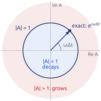
One step of a linear scheme applied to \(d\psi/dt = i\omega\psi\) multiplies \(\psi\) by a complex number, the amplification factor \(A\): \[ \psi^{n+1} = A\,\psi^n, \qquad \psi^n = A^n\psi^0, \] with \(\psi^n\) the amplitude at \(t^n = n\Delta t\). The exact solution has \(A = e^{i\omega\Delta t}\), on the unit circle at the angle \(\omega\Delta t\) (Figure 8). If \(|A| > 1\) the mode grows: the scheme is unstable; if \(|A| < 1\) it decays, damped; if \(|A| = 1\) it keeps its amplitude, like the waves. The angle of \(A\) compared with \(\omega\Delta t\) is the phase error of one step. Small departures add up: with \(|A| = 1.01\), a thousand steps multiply the amplitude by \(1.01^{1000} \approx 2\times10^4\). A scheme for waves is therefore judged by its \(A\) on the oscillation equation: its size (amplitude) and its angle (phase) (Durran 2010, sec. 2.2).
9 Amplification (1/3): forward Euler
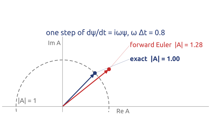
Forward Euler takes the slope at the start of the step: \[ \psi^{n+1} = \psi^n + \Delta t\,(i\omega\psi^n), \qquad A = 1 + i\omega\Delta t, \qquad |A| = \sqrt{1 + \omega^2\Delta t^2} > 1 . \] Every oscillation grows, for every \(\Delta t > 0\): forward Euler is unconditionally unstable for waves. The step follows the tangent of the circle and leaves it (Figure 9). The growth per oscillation period, \(|A|^{2\pi/(\omega\Delta t)} \approx e^{\pi\omega\Delta t}\), tends to 1 as \(\Delta t \to 0\): a smaller step grows more slowly, but never not at all. The angle is also wrong: \(\arg A = \arctan(\omega\Delta t) < \omega\Delta t\) (Durran 2010, sec. 2.2; Cushman-Roisin and Beckers 2011, sec. 2.6).
10 Amplification (2/3): backward, trapezoidal
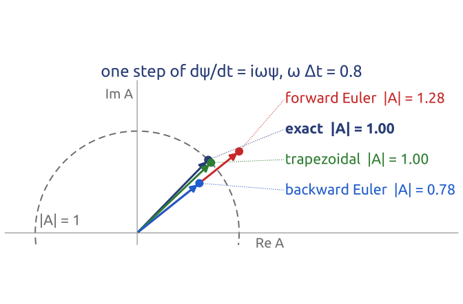
Backward Euler takes the slope at the end of the step, which makes it implicit: \[ \psi^{n+1} = \psi^n + \Delta t\,(i\omega\psi^{n+1}) \quad\Rightarrow\quad A = \frac{1}{1 - i\omega\Delta t}, \qquad |A| = \frac{1}{\sqrt{1 + \omega^2\Delta t^2}} < 1 : \] every oscillation is damped, the faster ones more. The trapezoidal scheme (Crank–Nicolson) averages the two slopes: \[ \psi^{n+1} = \psi^n + \frac{\Delta t}{2}\,i\omega\,(\psi^n + \psi^{n+1}) \quad\Rightarrow\quad A = \frac{1 + i\omega\Delta t/2}{1 - i\omega\Delta t/2}, \qquad |A| = 1 , \] neutral and second order, with a phase lag: \(\arg A = 2\arctan(\omega\Delta t/2) < \omega\Delta t\) (Figure 10). Both are stable for any \(\Delta t\), but for a whole grid each step requires solving a linear system for all the unknowns at the new time (Durran 2010, sec. 2.2.3). Semi-implicit models use the trapezoidal scheme for the gravity-wave terms only.
11 Amplification (3/3): leapfrog’s two roots
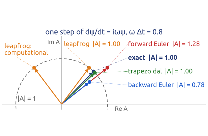
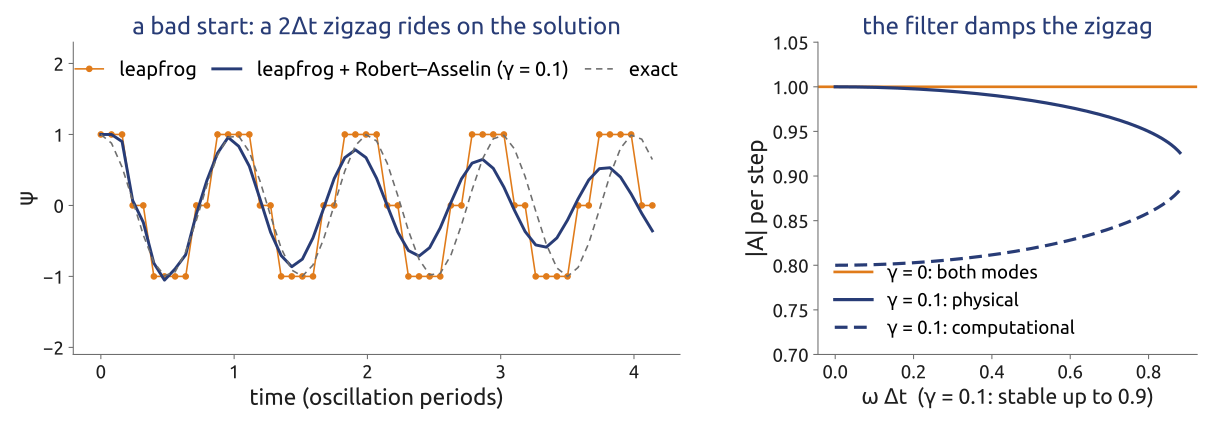
Leapfrog, Richardson’s step-over, is centred in time: \[ \psi^{n+1} = \psi^{n-1} + 2\Delta t\,(i\omega\psi^n). \] Trying \(\psi^n = A^n\psi^0\) gives a quadratic, with two roots, \[ A^2 - 2i\omega\Delta t\,A - 1 = 0 \quad\Rightarrow\quad A_\pm = i\omega\Delta t \pm \sqrt{1 - \omega^2\Delta t^2}. \] For \(|\omega\Delta t| < 1\), \(|A_\pm|^2 = \omega^2\Delta t^2 + (1 - \omega^2\Delta t^2) = 1\): leapfrog is neutral, explicit and second order. At \(|\omega\Delta t| = 1\) the two roots coincide; beyond it one root has \(|A| > 1\) and the scheme is unstable (Durran 2010, sec. 2.4.1). A scheme with three time levels has two solutions: \(A_+ \to e^{i\omega\Delta t}\) as \(\Delta t \to 0\), the physical mode, with the angle \(\arcsin(\omega\Delta t) > \omega\Delta t\) (slightly fast), while \(A_- \to -1\), the computational mode, a spurious zigzag of period \(2\Delta t\) (Figure 11). How much of it is present depends on how the scheme is started (leapfrog needs two initial levels; the first step is usually a forward step) and on whatever breaks the symmetry between even and odd steps: nonlinear terms, friction. Two-level schemes have one root and no computational mode.
12 The inertial oscillation with four schemes
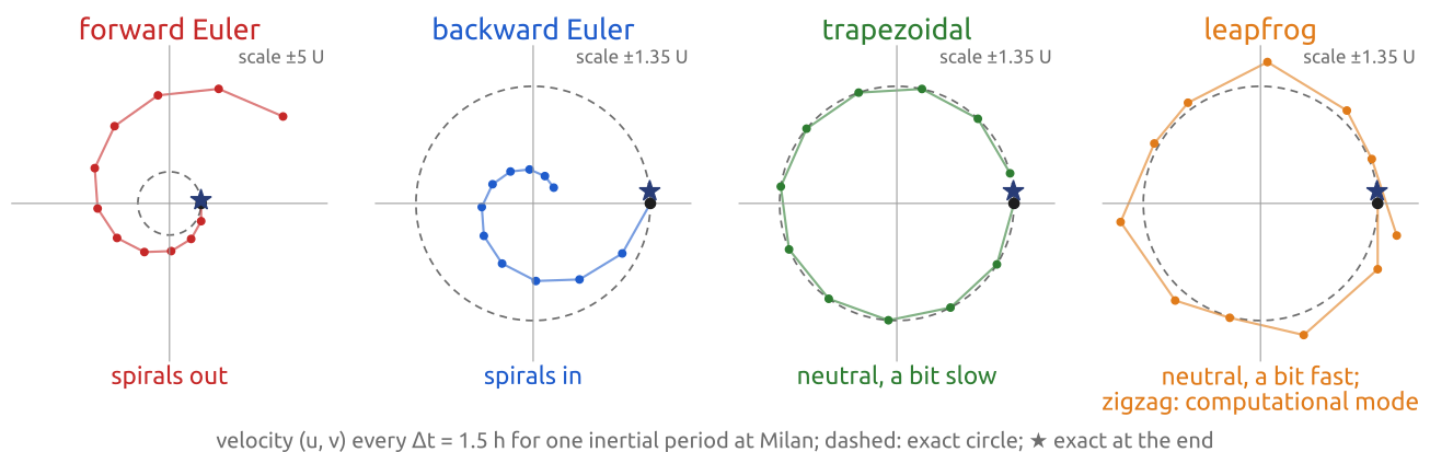
Figure 12 advances the inertial oscillation at Milan (\(f = 1.04\times10^{-4}\ \mathrm{s^{-1}}\)) with \(\Delta t = 1.5\) h, \(f\Delta t = 0.56\), for 11 steps, about one inertial period; the velocity should go once round the circle and keep its size. Forward Euler spirals out (\(|A| = 1.15\) per step, a factor 4.5 after 11 steps), backward Euler spirals in (0.22), the trapezoidal scheme stays on the circle but lags (2.5 % per step, \(2\arctan(f\Delta t/2)\) against \(f\Delta t\)), and leapfrog keeps its size but turns 6 % too fast (\(\arcsin(f\Delta t)\) against \(f\Delta t\)). Leapfrog’s first step, a forward-Euler step, splits the start between its two modes: the physical mode gets an amplitude 1.10 instead of 1, the computational mode 0.10, which shows as a zigzag about the circle. Same equation, same step: the scheme decides whether the current grows, dies or keeps its size (Cushman-Roisin and Beckers 2011, secs. 2.6–2.9, where the same schemes and their predictor–corrector variants are discussed; Durran 2010, sec. 2.2).
13 Leapfrog’s zigzag and the Robert–Asselin filter
Robert (1966) and Asselin (1972) proposed to follow each leapfrog step by a weak smoothing in time, \[ \bar\psi^n = \psi^n + \gamma\left(\bar\psi^{n-1} - 2\psi^n + \psi^{n+1}\right), \] where the bar marks filtered values, used in the next step, and \(\gamma\) is the filter coefficient. For the oscillation equation the two amplification factors become (Durran 2010, sec. 2.4.2, eq. 2.69) \[ A_\pm = \gamma + i\omega\Delta t \pm \sqrt{(1 - \gamma)^2 - \omega^2\Delta t^2}. \] At \(\omega\Delta t = 0\) the computational root is \(A_- = -(1 - 2\gamma)\): the zigzag is damped by the factor \(1 - 2\gamma\) per step. The physical mode is damped much less, \(|A_+| \approx 1 - \gamma(\omega\Delta t)^2/[2(1 - \gamma)]\), but the scheme becomes first order. For well-resolved slow motions this damping is negligible; for the fastest waves of a model it is not: with \(\gamma = 0.1\) and \(\omega\Delta t = 0.5\) the amplitude halves in four periods (Figure 13). Values \(\gamma \approx 0.06\) are typical in global models; with \(\gamma = 0.1\), stability requires \(|\omega\Delta t| \le 0.9\). Leapfrog with the Robert–Asselin filter ran most weather and climate models for decades; many now use Runge–Kutta schemes.
14 Runge–Kutta schemes and stability regions
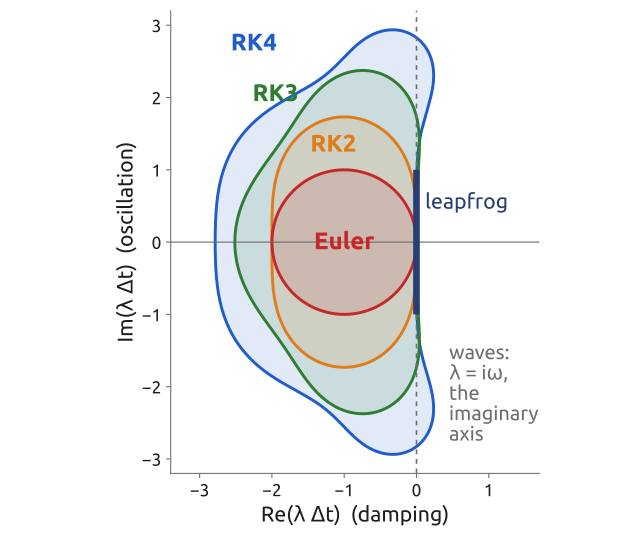
Runge–Kutta schemes evaluate the tendency at several intermediate stages within one step and combine them. They keep one time level, so they have no computational mode. The three-stage scheme of Wicker and Skamarock (2002), used in MPAS, reads for \(d\psi/dt = F(\psi)\) \[ \psi^* = \psi^n + \frac{\Delta t}{3}F(\psi^n), \qquad \psi^{**} = \psi^n + \frac{\Delta t}{2}F(\psi^*), \qquad \psi^{n+1} = \psi^n + \Delta t\,F(\psi^{**}). \] On \(F = \lambda\psi\), with \(z = \lambda\Delta t\), the stages give \(\psi^* = (1 + z/3)\psi^n\), \(\psi^{**} = (1 + z/2 + z^2/6)\psi^n\) and \[ A_{\mathrm{RK3}} = 1 + z + \frac{z^2}{2} + \frac{z^3}{6}, \] the Taylor polynomial of \(e^z\) of degree 3: the scheme is third order for linear problems (Skamarock et al. 2012). The classical schemes of order \(s = 1\) to 4 with \(s\) stages have the same form up to \(z^s/s!\); RK4 adds \(z^4/24\). Their stability regions, the sets of \(z\) with \(|A(z)| \le 1\), are drawn in Figure 14. Damping has \(z\) on the negative real axis, waves on the imaginary axis, \(z = i\omega\Delta t\). Forward Euler and RK2 contain no piece of the imaginary axis: they amplify all waves, slightly for small \(\omega\Delta t\). RK3 is stable for \(|\omega\Delta t| \le \sqrt3\) and RK4 for \(|\omega\Delta t| \le 2\sqrt2\) (Durran 2010, sec. 2.3). Each stage costs one evaluation of the tendency, so the useful measure is the largest stable step per stage. Explicit schemes for waves are stable only for \(|\omega\Delta t|\) below a limit of order one, and the fastest wave, with the largest \(\omega\), sets the step.
15 In class: forward Euler on the inertial oscillation
Exercise 1 — Forward Euler on the inertial oscillation. With \(w = u + iv\) the inertial oscillation \(du/dt = fv\), \(dv/dt = -fu\) is \(dw/dt = -ifw\). (a) One forward-Euler step multiplies \(w\) by a number \(A\): find \(A\) and \(|A|\). (b) At Milan (\(f = 1.04\times10^{-4}\,\mathrm{s^{-1}}\)) with \(\Delta t = 1\) h: by how much has the speed \(|w|\) grown after one inertial period, \(2\pi/f \approx 16.8\) h?
(c) To hand in: friction, and leapfrog. (i) Add a linear friction (drag) with rate \(r = 1/(1\ \text{day})\): \(dw/dt = -(if + r)\,w\). Find \(|A|\) for forward Euler. Can friction save it? For which \(\Delta t\) does the speed stop growing at Milan? (ii) Without friction, leapfrog: \(w^{n+1} = w^{n-1} - 2if\Delta t\,w^n\) (try \(w^n = A^n\)). What is the longest step at Milan that does not blow up? Which scheme would you use for the inertial currents of an ocean model, and why?
16 What the exercise showed
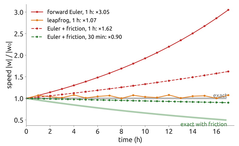
- For \(dw/dt = -ifw\), forward Euler gives \(A = 1 - if\Delta t\) and \(|A| = \sqrt{1 + (f\Delta t)^2}\). (b) At Milan with \(\Delta t = 1\) h, \(f\Delta t = 0.374\) and \(|A| = 1.068\); one inertial period is 16.8 steps, and \(1.068^{16.8} \approx 3.0\): the speed triples (Figure 15).
(c)(i) With a linear friction of rate \(r = 1/(1\ \text{day})\), \(dw/dt = -(if + r)w\) and \(A = 1 - (r + if)\Delta t\), so \(|A|^2 = (1 - r\Delta t)^2 + (f\Delta t)^2\). This is at most 1 only if \(\Delta t \le 2r/(r^2 + f^2) \approx 2100\) s, 35 min; with 1 h the speed still grows (by 1.6 in one period), and even with 30 min it decays more slowly than the true solution, \(e^{-rt}\). Friction does not save forward Euler on waves. (ii) Without friction, leapfrog, \(w^{n+1} = w^{n-1} - 2if\Delta t\,w^n\), gives \(A^2 + 2if\Delta t\,A - 1 = 0\), whose roots have \(|A| = 1\) for \(f\Delta t \le 1\): steps up to \(1/f = 2.7\) h at Milan. For the inertial currents of an ocean model one uses a neutral scheme, leapfrog with a filter or RK3, not forward Euler (Cushman-Roisin and Beckers 2011, secs. 2.6–2.9; Durran 2010, sec. 2.2).
17 Accuracy and stability, measured
The schemes of the previous sections can be run on one ordinary differential equation and their properties measured. Halving the step divides the error of forward Euler by 2.0, of RK2, RK3 and RK4 by 4.05, 8.26 and 15.98: the orders 1 to 4. On a decaying equation, \(d\psi/dt = \lambda\psi\) with \(\lambda\) real and negative, the amplification factors of the stability regions predict when each scheme blows up; on the oscillation equation the largest stable steps of RK3 and RK4 come out as \(|\omega\Delta t| = 1.732\) and \(2.828\), \(\sqrt3\) and \(2\sqrt2\). On the inertial oscillation, six schemes (forward and backward Euler, trapezoidal, leapfrog, RK3, RK4) reproduce the paths of Figure 12; forward Euler with \(\Delta t = 1\) h multiplies the speed by 3.05 after 17 steps, exactly \(|A|^{17}\), and leapfrog stays bounded for \(f\Delta t = 0.95\) but grows by \(10^8\) at \(f\Delta t = 1.05\). The Runge–Kutta scheme of MPAS (Wicker and Skamarock 2002) divides its error by 8.00 when the step is halved on a linear problem, but only by about 4 on a nonlinear one: it is third order only for linear problems.
18 Accuracy and stability are different properties
- Order. The error of forward Euler halves when \(\Delta t\) halves; RK3 divides it by 8, RK4 by 16.
- Stability is a separate question. On \(d\psi/dt = -60\psi\), forward Euler has \(A = 1 - 60\Delta t\), and \(|A| \le 1\) requires \(\Delta t \le 1/30\): beyond that it blows up, however accurate it is for small \(\Delta t\).
- Waves. Only schemes whose stability region holds a piece of the imaginary axis survive long integrations of waves: leapfrog, RK3, RK4, trapezoidal.
- Cost. Stages are not free; what matters is the largest stable step per stage.
So far the question was time only. When a whole field moves across the grid, the errors of the space differences and of the time steps meet: advection (Durran 2010, secs. 2.1–2.3).
19 Advection: the simplest transport
The simplest transport problem is the advection of a tracer \(q\) (humidity, salt) at constant speed \(c > 0\), \[ \frac{\partial q}{\partial t} + c\,\frac{\partial q}{\partial x} = 0, \qquad q(x, t) = q_0(x - ct), \] whose solution is the initial profile translated without change. With the Courant number \(C = c\,\Delta t/\Delta x\), four classical schemes are (Durran 2010, sec. 3.4):
- upwind (forward in time, backward in space, for \(c > 0\): the difference on the side the flow comes from): \(q_j^{n+1} = q_j^n - C\,(q_j^n - q_{j-1}^n)\);
- forward in time, centred in space (FTCS, the name used by Kalnay (2003)): \(q_j^{n+1} = q_j^n - \tfrac{C}{2}(q_{j+1}^n - q_{j-1}^n)\);
- leapfrog, centred in both: \(q_j^{n+1} = q_j^{n-1} - C\,(q_{j+1}^n - q_{j-1}^n)\);
- Lax–Wendroff (Lax and Wendroff 1960): expand in time, \(q^{n+1} = q^n + \Delta t\,\partial_t q + \tfrac{\Delta t^2}{2}\partial_t^2 q\), replace \(\partial_t q = -c\,\partial_x q\) and \(\partial_t^2 q = c^2\,\partial_x^2 q\), and use centred differences: \(q_j^{n+1} = q_j^n - \tfrac{C}{2}(q_{j+1}^n - q_{j-1}^n) + \tfrac{C^2}{2}(q_{j+1}^n - 2q_j^n + q_{j-1}^n)\), second order in time and space.
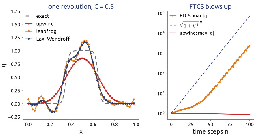
Run for one revolution round a periodic domain with \(C = 0.5\) and 50 points (Figure 16), upwind smears the profile, leapfrog and Lax–Wendroff keep its height but leave wiggles, and FTCS blows up, although it is centred and consistent. Why?
20 Von Neumann (1/3): one Fourier mode at a time
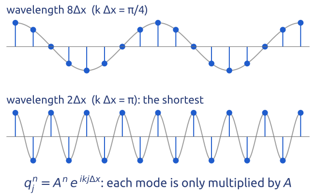
On a periodic grid, any grid function is a finite sum of Fourier modes \(e^{ikx_j}\) with \(\theta = k\Delta x \in [-\pi, \pi]\); the shortest one, \(\theta = \pi\), has wavelength \(2\Delta x\) (Figure 17). For a linear scheme with constant coefficients each mode evolves on its own, multiplied at each step by its amplification factor (Durran 2010, sec. 3.2.2): \[ q_j^n = A^n\,e^{\,ikj\Delta x}. \] Putting this into the scheme and dividing by \(A^n e^{ikj\Delta x}\) gives an equation for \(A(\theta)\). The scheme is stable, in this sense, if \(|A(\theta)| \le 1\) for every \(\theta\). Charney et al. (1950) (section V) used this Fourier analysis for the ENIAC forecast, “patterned after” Courant, Friedrichs and Lewy. The shortest modes are often the first to blow up.
21 Von Neumann (2/3): upwind is stable for \(C \le 1\)
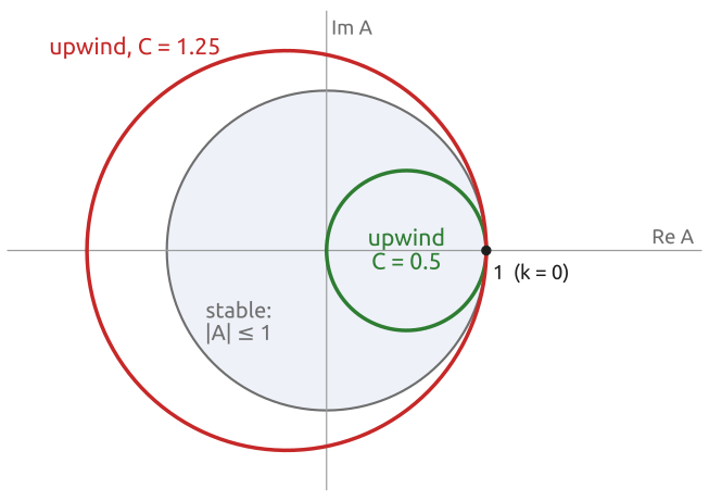
Put the mode into the upwind scheme: \[ A\,e^{ikj\Delta x} = e^{ikj\Delta x} - C\left(e^{ikj\Delta x} - e^{ik(j-1)\Delta x}\right) \quad\Rightarrow\quad A = 1 - C + C\,e^{-i\theta}, \] and \(|A|^2 = 1 - 2C(1 - C)(1 - \cos\theta)\). As \(\theta\) varies, \(A\) runs round a circle of radius \(C\) centred at \(1 - C\); it lies inside the unit circle if and only if \(0 \le C \le 1\) (Figure 18). For \(C = 1\), \(A = e^{-i\theta}\): the scheme reduces to \(q_j^{n+1} = q_{j-1}^n\), an exact shift by one cell. Upwind is stable if the flow crosses at most one cell per step.
22 Von Neumann (3/3): FTCS is always unstable
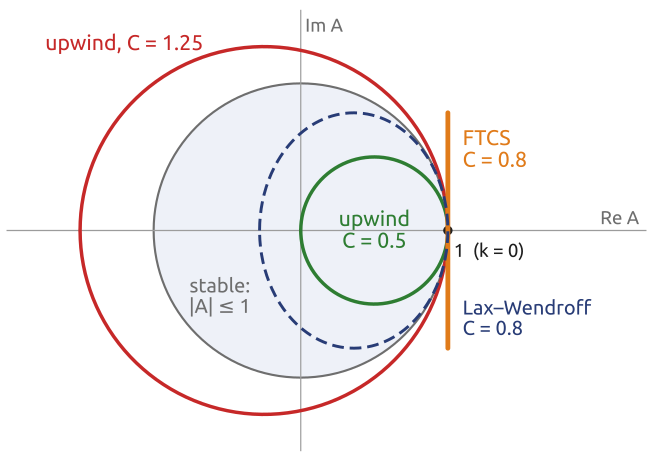
For FTCS, with \(\theta = k\Delta x\), \[ A = 1 - iC\sin\theta, \qquad |A|^2 = 1 + C^2\sin^2\theta > 1 \quad (C > 0): \] a vertical segment through 1, outside the unit circle for every time step (Figure 19). The centred difference gives imaginary eigenvalues, a pure oscillation, and forward Euler amplifies every oscillation (Section 9). The worst mode, \(\theta = \pi/2\) (wavelength \(4\Delta x\)), grows by \(\sqrt{1 + C^2}\) per step, as in the run of Figure 16. Lax–Wendroff adds the term \(-C^2(1 - \cos\theta)\): \[ A = 1 - iC\sin\theta - C^2(1 - \cos\theta), \qquad |A|^2 = 1 - C^2(1 - C^2)(1 - \cos\theta)^2, \] an ellipse back inside the unit circle for \(C \le 1\). Leapfrog gives \(A^2 + 2iC\sin\theta\,A - 1 = 0\), so \(A = -iC\sin\theta \pm \sqrt{1 - C^2\sin^2\theta}\): neutral for \(C < 1\), with a computational mode; at \(C = 1\) the roots coincide and a weakly unstable \(4\Delta x\) wave appears (Durran 2010, sec. 3.2.2, §3.4.4). Consistency is not enough: FTCS approximates the equation and still blows up.
23 Eigenvalues on the stability regions
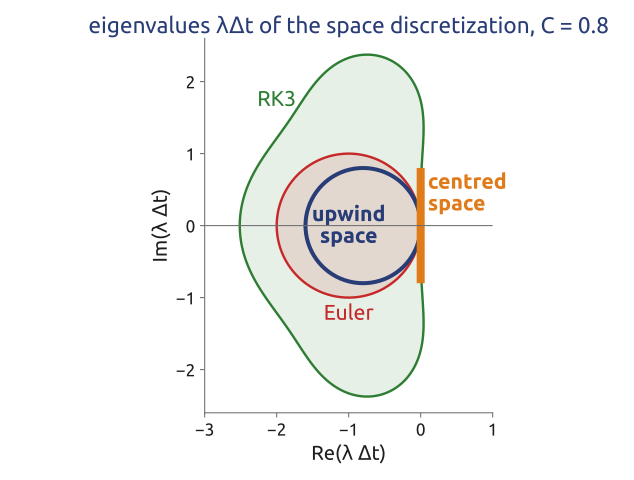
The same results follow from the method of lines. The space difference alone turns the advection equation into \(d\mathbf q/dt = \mathsf L\mathbf q\), whose eigenvalues, for the Fourier mode \(\theta\), are \(\lambda(\theta)\); the full scheme is stable when every \(\lambda\Delta t\) lies in the stability region of the time scheme (Figure 20) (Durran 2010, sec. 2.2.4). The upwind difference has \(\lambda\Delta t = -C(1 - e^{-i\theta})\), a circle of radius \(C\) centred at \(-C\) in the left half-plane: it damps, and it fits inside Euler’s disk if \(C \le 1\). The centred difference has \(\lambda\Delta t = -iC\sin\theta\), a segment of the imaginary axis: a pure oscillation, never stable with forward Euler (FTCS), stable with leapfrog if \(C \le 1\), with RK3 if \(C \le \sqrt3\), with RK4 if \(C \le 2\sqrt2\). The fastest wave sets the largest \(|\lambda|\), \(c/\Delta x\) times a factor of order one, so the limit is always on \(C\). The time-stepping picture and von Neumann’s are the same picture.
24 Courant, Friedrichs and Lewy (1928)
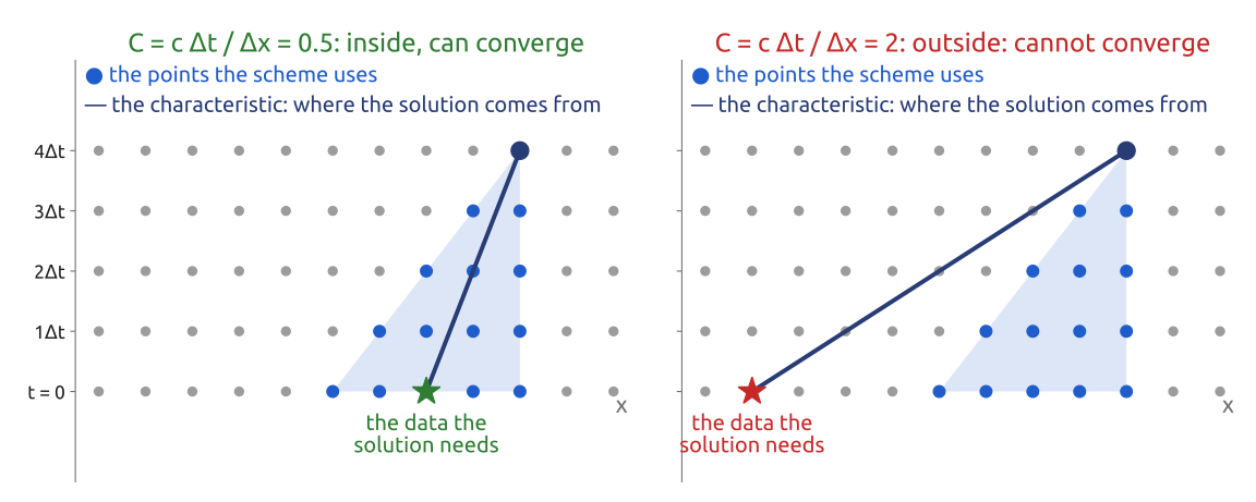
Courant et al. (1928) observed that the solution of the advection equation at \((x_j, t^n)\) is the initial value at \(x_j - ct^n\), carried along the characteristic. An explicit scheme with a stencil of one neighbour on each side can only use initial data within \(n\) grid points of \(x_j\): its numerical domain of dependence. If the true domain of dependence lies outside it, changing the initial data there changes the true solution but not the computed one, and the scheme cannot converge, whatever its weights (Figure 21). For upwind this gives \(x_j - ct^n \ge x_{j-n}\), that is \[ C = \frac{c\,\Delta t}{\Delta x} \le 1 . \] For a system of equations \(c\) is the fastest wave speed: for the shallow water equations, \(|u| + \sqrt{gH}\) (Durran 2010, sec. 3.2.3). The CFL condition is necessary but not sufficient: FTCS satisfies it for \(C \le 1\) and is unstable. Courant, Friedrichs and Lewy wrote it for existence proofs, not for computers; Lynch (2008) recalls that von Neumann, who was in Göttingen in the 1920s, knew their work, and that at the 1946 Princeton meeting “it was clear that the CFL stability criterion prohibited the use of a long time step such as had been used by Richardson”.
25 Aside: the Lax–Richtmyer equivalence theorem
Let a linear initial-value problem be well posed, and a linear finite-difference scheme be consistent with it: its truncation error tends to zero as \(\Delta t, \Delta x \to 0\). Then the scheme converges if and only if it is stable, meaning that for every \(T\) there is a constant \(C_T\) with \(\|q^n\| \le C_T\,\|q^0\|\) for all \(n\Delta t \le T\), uniformly in \(\Delta t\) and \(\Delta x\) small enough (Lax and Richtmyer 1956; Durran 2010, sec. 3.2). A stable scheme accurate of order \((p, q)\) converges with error \(O(\Delta t^p) + O(\Delta x^q)\). Consistency is the hypothesis, checked with Taylor series; stability, checked with von Neumann’s method for constant coefficients on periodic grids, is then exactly what decides convergence. In general the stability condition allows \(|A| \le 1 + O(\Delta t)\). Consistency is not a necessary condition for convergence: on non-uniform grids a scheme can converge without it (supraconvergence). For nonlinear problems there is no such theorem, and conservation properties become important.
26 Advection, computed
The schemes of Section 19 can be run and their properties measured: upwind with \(C = 1\) (an exact shift), \(0.4\) (diffused) and \(1.2\) (unstable); the CFL picture, varying \(\Delta x\) and \(\Delta t\) separately to see that only their ratio \(C\) decides stability; six schemes side by side on the profile of Wicker and Skamarock (2002); and \(|A|\) measured on single Fourier modes against the formulas of the von Neumann sections. A modified equation (Section 27) can be checked by fitting the decay of the upwind run, and convergence by refining the grid at fixed \(C\).
27 Numerical diffusion
What equation does the upwind scheme actually solve? Expand every value in the scheme in Taylor series about \((x_j, t^n)\): \[ \frac{q_j^{n+1} - q_j^n}{\Delta t} + c\,\frac{q_j^n - q_{j-1}^n}{\Delta x} = \frac{\partial q}{\partial t} + \frac{\Delta t}{2}\frac{\partial^2 q}{\partial t^2} + c\,\frac{\partial q}{\partial x} - \frac{c\,\Delta x}{2}\frac{\partial^2 q}{\partial x^2} + O(\Delta t^2, \Delta x^2) = 0 . \] To leading order \(\partial_t q = -c\,\partial_x q\), so \(\partial_t^2 q = c^2\,\partial_x^2 q\) (to this order only; the substitution cannot be repeated for the higher terms, which is why Durran (2010), §3.4.2, eq. 3.67, keeps a third-derivative term, \(-\tfrac{c\,\Delta x^2}{6}(1 - C)(1 - 2C)\,\partial_x^3 q\)), and \[ \frac{\partial q}{\partial t} + c\,\frac{\partial q}{\partial x} = \frac{c\,\Delta x}{2}\,(1 - C)\,\frac{\partial^2 q}{\partial x^2} + O(\Delta t^2, \Delta x^2). \] This modified equation has a diffusion term that was never asked for: numerical diffusion, with the coefficient \(\tfrac{c\,\Delta x}{2}(1 - C)\). It smooths the profile and lowers its maximum (the upwind run of Figure 16), vanishes for \(C = 1\), and is negative, an anti-diffusion and an instability, for \(C > 1\) (Durran 2010, sec. 3.3.2, §3.4.2). For a wind of 10 m/s on a 100 km grid with \(C = 0.5\) it is \(2.5\times10^5\ \mathrm{m^2\,s^{-1}}\), much larger than any physical diffusion at these scales.
Centred schemes, leapfrog and Lax–Wendroff, keep the amplitude better but leave wiggles: they have no second-derivative error term, and their leading error is a third derivative, \(\partial^3 q/\partial x^3\), which does not damp but makes waves of different lengths travel at different speeds: dispersion.
28 Phase speed: the \(2\Delta x\) wave stands still
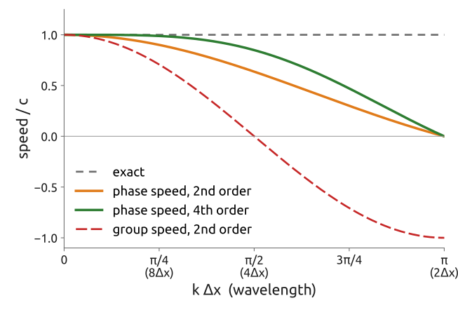
For the centred difference without time discretization, a mode \(e^{i(kx - \omega t)}\) satisfies \(-i\omega = -c\,(e^{ik\Delta x} - e^{-ik\Delta x})/(2\Delta x) = -ic\sin(k\Delta x)/\Delta x\), so \[ \omega = \frac{c\,\sin(k\Delta x)}{\Delta x}, \qquad \frac{c^*}{c} = \frac{\sin(k\Delta x)}{k\Delta x}, \qquad c_g = \frac{d\omega}{dk} = c\cos(k\Delta x), \] with \(c^* = \omega/k\) the phase speed on the grid and \(c_g\) its group speed (Durran 2010, sec. 3.3.1). (For the oscillation equation \(\psi \propto e^{i\omega t}\); for waves \(e^{i(kx - \omega t)}\): the conventions differ by the sign of \(\omega\), which does not matter for stability.) Long waves, \(k\Delta x \ll 1\), move at nearly the right speed; short waves are too slow; the \(2\Delta x\) wave, \(k\Delta x = \pi\), does not move at all; and for waves shorter than \(4\Delta x\) the group speed is negative: their energy travels backwards, which is why the wiggles appear behind the moving profile (Figure 22). The fourth-order centred difference, \(c^*/c = (8\sin k\Delta x - \sin 2k\Delta x)/(6k\Delta x)\), improves the intermediate waves but not the shortest. A rule of thumb: a feature needs 8–10 grid points per wavelength to move at about the right speed (Randall 2011). Spectral methods give the exact speed for every wave the grid resolves.
29 A and C grids (1/2): where \(h\) and \(u\) live
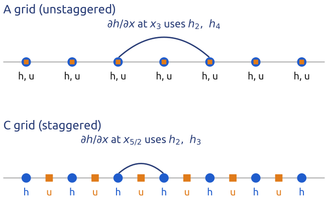
The linear gravity waves of Section 7, written for the height of the surface \(h = H + \eta\) (with a flat bottom \(\partial h = \partial\eta\)), \[ \frac{\partial h}{\partial t} + H\,\frac{\partial u}{\partial x} = 0, \qquad \frac{\partial u}{\partial t} + g\,\frac{\partial h}{\partial x} = 0, \] couple two variables: the tendency of each needs the derivative of the other. Two arrangements of the unknowns on a uniform grid are compared (Figure 23) (Mesinger and Arakawa 1976; Durran 2010, sec. 4.1.2):
- A grid (unstaggered): \(h_j\) and \(u_j\) at the same points \(x_j\); centred differences over \(2\Delta x\), \((\partial h/\partial x)_j \approx (h_{j+1} - h_{j-1})/(2\Delta x)\).
- C grid (staggered): \(h_j\) at \(x_j\), \(u_{j+1/2}\) half-way between; differences over \(\Delta x\), \((\partial h/\partial x)_{j+1/2} \approx (h_{j+1} - h_j)/\Delta x\) and \((\partial u/\partial x)_j \approx (u_{j+1/2} - u_{j-1/2})/\Delta x\).
Both carry two unknowns per \(\Delta x\). Staggering puts each derivative where it is needed, at the shortest distance. Does it matter?
30 A and C grids (2/2): the \(2\Delta x\) mode
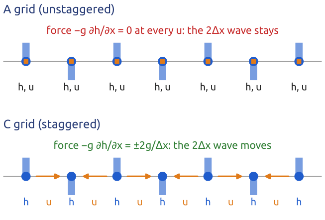
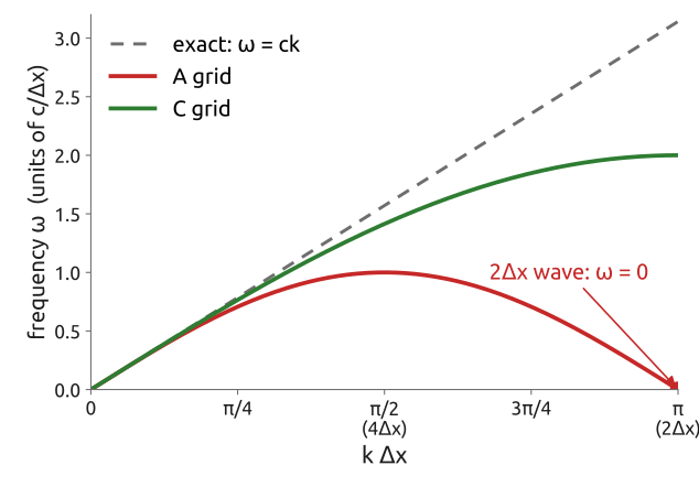
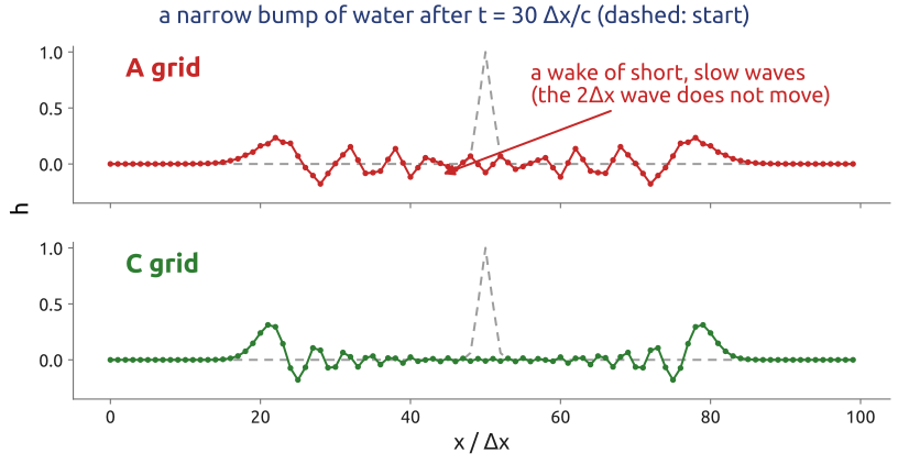
With \(h, u \propto e^{i(kx - \omega t)}\) and \(c = \sqrt{gH}\), the A grid gives \(-i\omega\hat h = -iH\hat u\sin(k\Delta x)/\Delta x\) and \(-i\omega\hat u = -ig\hat h\sin(k\Delta x)/\Delta x\); on the C grid each centred difference over \(\Delta x\) brings \(2i\sin(k\Delta x/2)/\Delta x\). Hence \[ \text{A grid: } \omega = \frac{c}{\Delta x}\,\sin(k\Delta x), \qquad \text{C grid: } \omega = \frac{2c}{\Delta x}\,\sin\frac{k\Delta x}{2}, \] against \(\omega = ck\) exactly (Figure 25). On the A grid the frequency rises to a maximum at \(k\Delta x = \pi/2\) and falls back to zero at the \(2\Delta x\) wave: a checkerboard \(h = +1, -1, +1, \dots\) has a zero centred gradient everywhere, so it exerts no force on \(u\) and simply stays, as noise (Figure 24); waves shorter than \(4\Delta x\) have a negative group speed. On the C grid the frequency increases monotonically, the group speed is positive for every resolved wave, and the checkerboard feels the largest force on the grid. This is why most models put their gravity waves on staggered grids; with rotation the choice is subtler, and depends on the ratio of the deformation radius to the grid spacing (Mesinger and Arakawa 1976; Randall 2011). The largest frequency of the C grid, \(2c/\Delta x\), sets its time step: leapfrog needs \(c\,\Delta t/\Delta x \le 1/2\).
31 The shallow water solver, opened
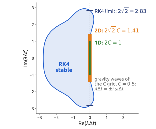
The shallow water solver used so far as a black box, for the waves and the geostrophic adjustment, is made of the pieces of this lecture: a C grid (\(\eta\) at cell centres, \(u\) and \(v\) on the faces), centred differences over one grid interval, the Coriolis terms from averages of the neighbouring velocities, and the classical RK4 scheme with \(\Delta t = 0.5\,\Delta x/c\), that is \(C = 0.5\). Is this step stable? The fastest wave of the C grid is the checkerboard: \(\omega_{\max} = 2c/\Delta x\) in one dimension and, in two with \(\Delta x = \Delta y\), the diagonal checkerboard, \(\omega_{\max} = 2\sqrt2\,c/\Delta x\). Rotation does not raise these values: the averaged Coriolis term vanishes for the checkerboard, so the \(f^2\) of the inertia–gravity frequency is multiplied by zero there (Randall 1994). Hence \(\omega_{\max}\Delta t = 2C = 1\) in 1D and \(2\sqrt2\,C = 1.41\) in 2D, both inside RK4’s interval \(|\omega\Delta t| \le 2\sqrt2 = 2.83\) (Figure 26): the solver is stable with a margin of 2 to 3, and would fail beyond \(C = \sqrt2\) in 1D or \(C = 1\) in 2D (Durran 2010, sec. 2.2.4, §4.1.2). RK4’s \(|A|\) is slightly below 1 on the imaginary axis, so the energy decreases slowly, by 0.2 % in four days. A grid, a difference, a time scheme and a step: each choice can now be checked on paper.
32 Shallow water in 1D, computed
The same solver can be written in one dimension and taken apart: the C grid, the three-stage Runge–Kutta scheme of Wicker and Skamarock (2002), a bump of water that adjusts geostrophically, a test that a balanced state stays still, the largest stable time step, and the comparison of the A and C grids (Figure 27). On the C grid, RK3 is stable for \(c\,\Delta t/\Delta x \le \sqrt3/2\), with \(\Delta x\) the distance between \(h\) points (the largest frequency is \(2c/\Delta x\)); the A grid allows twice the step, but keeps its noisy short waves. The mass, computed from fluxes between cells, is conserved to round-off.
33 In class: why 1950 worked and 1922 did not
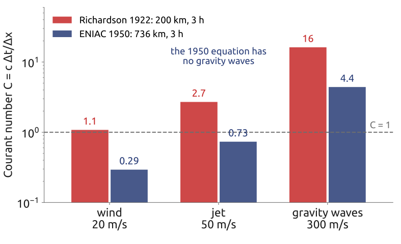
Exercise 2 — Why 1950 worked and 1922 did not. Compute the Courant number \(C = c\,\Delta t/\Delta x\) of Richardson’s forecast (grid about 200 km, leapfrog step \(\Delta t = 3\) h) and of the ENIAC forecast (\(\Delta x = 736\) km, \(\Delta t = 3\) h) for a wind of 20 m/s, a jet of 50 m/s and gravity waves at 300 m/s. Which signals could each scheme follow? Why could the ENIAC ignore the gravity waves?
(c) To hand in: an ocean model. A model with \(\Delta x = 10\) km over an ocean 4000 m deep: what is the longest explicit time step allowed by the surface gravity waves (\(c = \sqrt{gH}\), take \(C \le 1\))? And by currents of 1 m/s? How many steps per day does each need? What would you do?
34 What the exercise showed
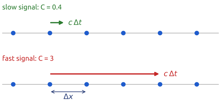
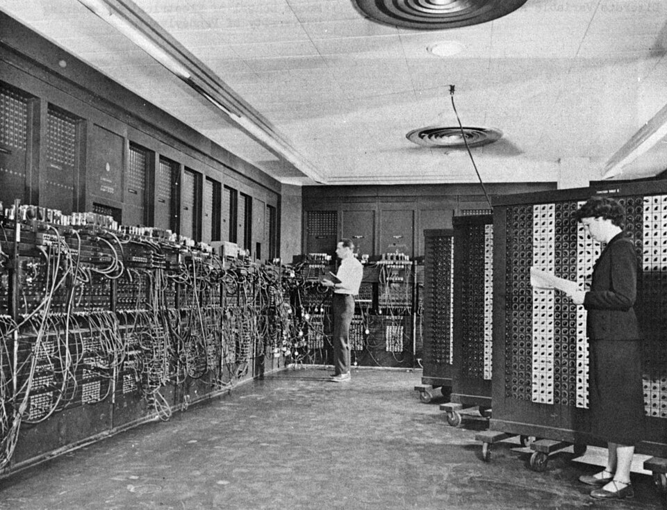
The Courant number \(C = c\,\Delta t/\Delta x\) counts the grid intervals a signal crosses in one step (Figure 28). Richardson’s 3-hour step on a 200 km grid gives \(C = 1.1\) for a wind of 20 m/s, 2.7 for a jet of 50 m/s and 16 for gravity waves at 300 m/s: no explicit scheme can follow them, and even with balanced data his forecast could not have been continued. The ENIAC forecasts of Charney et al. (1950) used a grid of \(15\times18\) intervals of 736 km on a polar stereographic map and time steps of first one, then two and three hours, “when it was found that the larger intervals gave practically identical forecasts and did not lead to computational instability”: with \(\Delta t = 3\) h, \(C = 0.29\) for the wind and \(0.73\) for the jet (Figure 29). The barotropic vorticity equation has no gravity waves, so their \(C = 4.4\) never arises; had they integrated the primitive equations, “the computational stability condition states that the ratio of the space to the time difference must exceed the gravitational wave velocity, about 300 m sec\(^{-1}\), and demands a time increment of some 15 minutes or less” (Charney et al. 1950), a hundred steps for 24 hours, too many for the ENIAC (Figure 30).
- An ocean model with \(\Delta x = 10\) km over 4000 m of water has surface gravity waves at \(c = \sqrt{gH} = 198\) m/s: \(C \le 1\) needs \(\Delta t \le 50\) s, about 1700 steps a day. Currents of 1 m/s alone would allow \(10^4\) s, 9 steps a day. Models therefore treat the fast waves apart: with short steps for the fast mode only (split-explicit), or implicitly. The fastest wave sets the explicit time step: filter it, split it, or treat it implicitly (Lynch 1999).

35 Key points
- Order: a difference’s error falls like \(\Delta x^p\) (Taylor series); centred differences have \(p = 2\).
- Stability: \(|A| \le 1\) for every mode (von Neumann); forward Euler amplifies waves; leapfrog is neutral but has a computational mode; RK3 and RK4 hold a piece of the imaginary axis.
- CFL: explicit schemes need \(C = c\,\Delta t/\Delta x \lesssim 1\): the fastest wave (gravity) sets \(\Delta t\). Necessary, not sufficient.
- Diffusion and dispersion: upwind smooths; centred schemes slow the short waves; the \(2\Delta x\) wave does not move.
- Staggering: on the C grid gravity waves have no \(2\Delta x\) null mode.
Richardson’s method was the right one; his time step was not: the fastest wave sets \(\Delta t\).
Further reading
Durran (2010), Chapters 2–4, is the reference for everything in this lecture: time stepping (Ch. 2), advection, von Neumann’s analysis, the CFL condition and the modified equation (Ch. 3), and staggered grids (§4.1). Cushman-Roisin and Beckers (2011) pairs each physical chapter with its numerics (§2.6–2.9 for time stepping). Döös et al. (2022) is a short open-access introduction; Randall (2011) discusses grids and dispersion with many examples; Mesinger and Arakawa (1976) is the classic report on the methods of atmospheric models. History: Lynch (1999) and Lynch (2008) for Richardson’s forecast and the road to the ENIAC.