November 2026 · Politecnico di Milano

Finite differences: time stepping, advection and the CFL condition

Atmosphere and Ocean Dynamics — Lecture 5

Prof. Dr. Pedro da Silva Peixoto

Applied Mathematics
Instituto de Matemática e Estatística
Universidade de São Paulo

Visiting Professor at MOX Lab
Politecnico di Milano

Warm-up

1. A tracer \(q\) (humidity, salt) carried by a constant wind \(c\): write its equation. What is the exact solution?
2. The inertial oscillation, \(du/dt = fv\), \(dv/dt = -fu\): write it as one equation for \(w = u + iv\). How does \(|w|\) change in time?
3. Write the linear shallow water equations in one dimension, with rotation, for \(\eta\), \(u\) and \(v\).
4. How fast are gravity waves in an ocean 4000 m deep? In the atmosphere (\(H \approx 8\) km)? And the ocean’s first baroclinic mode, \(c_1 = NH/\pi\), with \(N = 2\times10^{-3}\) s\(^{-1}\)?
5. The 1950 forecast and the vertical slice step a vorticity forward in time. What must they also solve at every step?

Lectures 1–4, from memory: answer on paper first, 3 minutes. These are the equations today’s numerics discretize. Today: how a computer steps them, and why it can blow up.

1. dq/dt + c dq/dx = 0 (partial derivatives); q(x, t) = q0(x - ct): the shape moves unchanged.
2. dw/dt = -i f w, so w = w0 exp(-i f t): |w| stays constant; the velocity turns clockwise, period 2 pi/f (16.8 h at Milan). 3. d(eta)/dt + H du/dx = 0, du/dt - f v = -g d(eta)/dx, dv/dt + f u = 0.
3. c = sqrt(gH): 198 m/s; 280 m/s (about 300); c_1 = 0.002 x 4000/pi = 2.5 m/s: the fastest wave sets the explicit time step. 5. A Poisson problem, lap(psi) = zeta (xi in the slice), for the streamfunction.

Where we are and where we are going

Previous knowledge

• Advection, \(\partial_t q + c\,\partial_x q = 0\): \(q = q_0(x - ct)\), the shape moves unchanged
• The inertial oscillation, \(w = u + iv\): \(dw/dt = -ifw\); \(|w|\) stays, period \(2\pi/f\) = 16.8 h at Milan
• Linear shallow water in 1D: \(\partial_t\eta + H\partial_x u = 0\), \(\partial_t u - fv = -g\partial_x\eta\), \(\partial_t v + fu = 0\)
• Gravity waves at \(\sqrt{gH}\): 200 m/s (ocean), 280 m/s (atmosphere); first baroclinic mode of the ocean \(NH/\pi \approx 2.5\) m/s
• The 1950 forecast and the slice: a Poisson problem \(\nabla^2\psi = \zeta\) at every step
• Taylor series, eigenvalues, complex numbers, Fourier series; a shallow water solver, so far a black box

Where we are going

1. Space first, then time: Taylor series
2. Time steps: amplification and stability
3. Leapfrog, Runge–Kutta, notebook
4. Advection: von Neumann and CFL
5. Notebook: numerical diffusion, dispersion
6. A and C grids; the solver opened
7. Why 1950 worked and 1922 did not

Accuracy and stability of a grid model, from one ODE to the shallow water equations

(Durran 2010, Ch. 1–4; Döös et al. 2022)

Two minutes. Left: what we take as known (lectures 1–4; the warm-up checked it); the black box is lecture 3’s notebook solver. Right: the road of the day; each item links to its first slide.

Richardson (1922): the method, and a time step

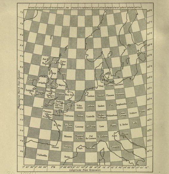
Richardson’s grid over Europe. Richardson (1922), public domain

• Grid every \(3^\circ\) of longitude and \(1.8^\circ\) of latitude: about 200 km
• His “step-over” is today’s leapfrog: tendencies at 07 UTC, one 6-hour jump

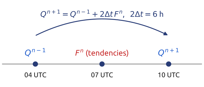
• Result: 145 hPa in 6 hours: the initial state was out of balance

But: with balanced data, could he have gone on, step after step?

A forecast by numbers needs a grid, a time step, and a scheme that does not blow up

(Richardson 1922; Lynch 1999) · Grid: archive.org/details/weatherpredictio00richrich

Recalls lecture 1 (the imbalance). Lynch (1999): the step was 3 h (2 dt = 6 h), “not six hours as so often stated”. Ask first: is a 3-hour step on a 200 km grid reasonable? We answer it at the end (exercise 2).

The method of lines: space first, then time

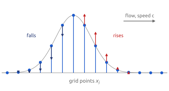
1. Space: keep the values \(q_j(t)\) at grid points \(x_j = j\,\Delta x\) and replace \(\partial q/\partial x\) by a difference of neighbours; for \(\partial_t q + c\,\partial_x q = 0\): \(\;\dfrac{dq_j}{dt} = -c\,\dfrac{q_{j+1} - q_{j-1}}{2\Delta x}\)
2. Each \(q_j\) now obeys an ordinary differential equation; all together:

\[\frac{d\mathbf{q}}{dt} = \mathbf{F}(\mathbf{q})\]

\(\mathbf q\): all the grid values \(q_j\); \(\mathbf F\): their tendencies, from the differences of neighbours

3. Time: step this system with \(\Delta t\), \(\;q_j^n \approx q(x_j, t^n)\)

Two questions for every scheme: how accurate is a difference, and is a time step stable?

(Durran 2010, sec. 1.3, sec. 3.3.1; Döös et al. 2022)

Figure: a bump moving right; each stem’s arrow is dq_j/dt from its neighbours (rises ahead, falls behind). Lecture 3’s “black box” solver is exactly this: space first, then a time scheme.

Taylor series (1/3): a derivative from grid values

Expand \(q\) around \(x_j\), one grid step ahead:

\[q_{j+1} = q_j + \Delta x\, q'_j + \frac{\Delta x^2}{2}\,q''_j + \frac{\Delta x^3}{6}\,q'''_j + \dots\]

and one step behind:

\[q_{j-1} = q_j - \Delta x\, q'_j + \frac{\Delta x^2}{2}\,q''_j - \frac{\Delta x^3}{6}\,q'''_j + \dots\]

Question: which combination of \(q_{j-1}, q_j, q_{j+1}\) best gives \(q'_j\)?

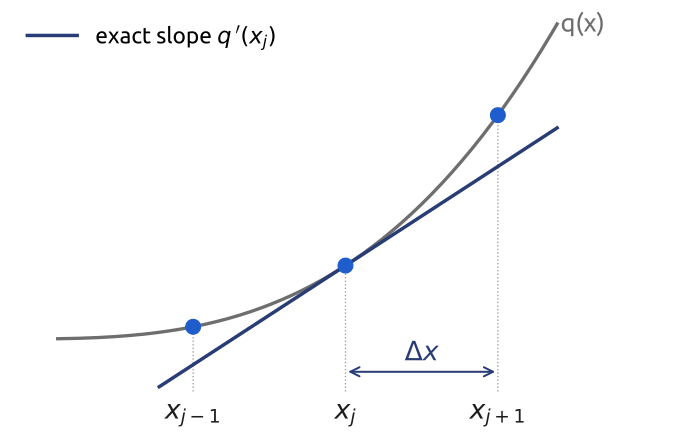
On a grid we only know values; derivatives must be built from them

(Durran 2010, sec. 1.3.1, sec. 3.1)

The board: write the two expansions, one below the other. Smooth q: Taylor applies.

Taylor series (2/3): forward difference

Solve the first expansion for \(q'_j\):

\[\frac{q_{j+1} - q_j}{\Delta x} = q'_j + {\color{#1f5ccc}\underbrace{\frac{\Delta x}{2}\,q''_j + \dots}_{\text{truncation error}}}\]

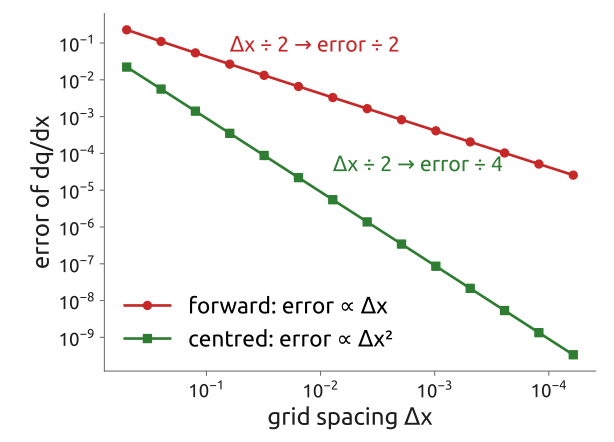
• The error goes to zero like \(\Delta x\): first order
• Halve \(\Delta x\), halve the error

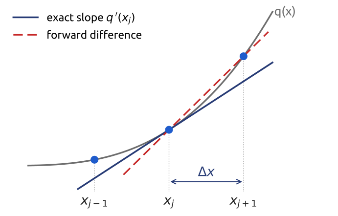
Truncation error: what the difference leaves out of the Taylor series

[Durran (2010), §3.1; §3.3.2, eq. 3.39]

Order p: error = C dx^p. Forward and backward are both first order.

Taylor series (3/3): centred is second order

Subtract the two expansions: the even terms cancel,

\[\frac{q_{j+1} - q_{j-1}}{2\Delta x} = q'_j + {\color{#1f5ccc}\frac{\Delta x^2}{6}\,q'''_j} + \dots\]

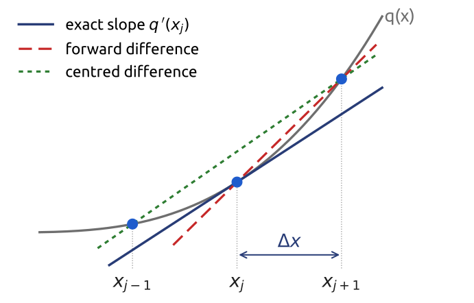
But: accurate at one instant is not enough. Do the errors grow when we step in time?

Order: the error falls like \(\Delta x^p\); centred differences are second order (\(p = 2\))

[Durran (2010), §3.1; §3.3.2, eq. 3.39; Döös et al. (2022)]

Log-log plot: slopes 1 and 2, computed for q = sin at x = 1. The centred line is nearly parallel to the tangent. A test for any code: halve dx, the error must drop by 2^p.

Normal modes: one equation for all waves

1. Linear gravity waves in 1D: \(\;\partial_t\eta + H\,\partial_x u = 0\), \(\;\partial_t u + g\,\partial_x\eta = 0\)
2. One Fourier mode, \((\eta, u) = (\hat\eta, \hat u)\,e^{ikx}\): a linear system, \[\frac{d}{dt}\begin{pmatrix}\hat\eta\\ \hat u\end{pmatrix} = \mathsf M\begin{pmatrix}\hat\eta\\ \hat u\end{pmatrix},\qquad \mathsf M = \begin{pmatrix}0 & -iHk\\ -igk & 0\end{pmatrix}\]
3. Its eigenvalues: \(\lambda^2 = -gHk^2\), so \(\lambda = \pm ick\), \(c = \sqrt{gH}\); eigenvectors \((\hat\eta, \hat u) = (H, \mp c)\): a wave going left, one going right

4. In the eigenvector basis each wave is on its own: the oscillation equation

\[\frac{d\psi}{dt} = \lambda\psi = i\omega\psi, \qquad \psi = \psi_0\,e^{i\omega t}\]

\(\psi\): the amplitude of one mode; \(\omega\): its frequency, here \(\pm ck\); \(|\psi|\) stays constant

• With rotation (\(v\), \(f\)): \(\lambda = 0\) (geostrophic) and \(\pm i\sqrt{f^2 + c^2k^2}\); at \(k = 0\), \(\pm if\): the inertial oscillation, \(dw/dt = -ifw\)
• Rossby waves: \(\lambda = i\omega\) too, with a small \(\omega\)

Every linear wave is one oscillation, \(d\psi/dt = i\omega\psi\): test a time scheme on it

(Durran 2010, sec. 2.2; Cushman-Roisin and Beckers 2011, sec. 2.7)

On the board: the 2x2 matrix, its characteristic polynomial, the eigenvectors (left: u = -c eta/H, right: u = +c eta/H). With rotation the 3x3 matrix gives the geostrophic mode and the Poincare waves (lecture 3). Assumes a diagonalizable M (normal modes), as for the linear shallow water equations.

The amplification factor

One step of a time scheme multiplies the mode by a number, the amplification factor \(A\):

\[\psi^{n+1} = A\,\psi^n, \qquad \psi^n = A^n\psi^0\]

\(\psi^n\): the amplitude at the time \(t^n = n\Delta t\). Exact: \(A = e^{i\omega\Delta t}\), on the unit circle

• \(|A| > 1\): grows, unstable
• \(|A| < 1\): decays, damped
• \(|A| = 1\): neutral, like the waves
• The angle of \(A\) against \(\omega\Delta t\): the phase error

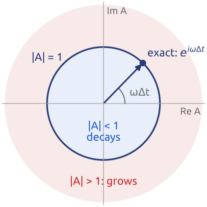
A scheme for waves is judged by its \(A\) on \(d\psi/dt = i\omega\psi\): size (amplitude) and angle (phase)

(Durran 2010, sec. 2.2; Cushman-Roisin and Beckers 2011, sec. 2.7)

Exact factor: A = exp(i w dt), on the unit circle, at the angle w dt. Inertial: w = -f, clockwise. Ask first: after n steps, what is the amplitude if |A| = 1.01? (1.01^n: after 1000 steps, 2.1e4.)

Amplification (1/3): forward Euler

Forward Euler: the slope at the start of the step,

\[\psi^{n+1} = \psi^n + \Delta t\,(i\omega\psi^n)\]

\[A = 1 + i\omega\Delta t, \qquad {\color{#1f5ccc}|A| = \sqrt{1 + \omega^2\Delta t^2} > 1}\]

• Every oscillation grows, for any \(\Delta t\)
• Smaller \(\Delta t\): slower growth, never none

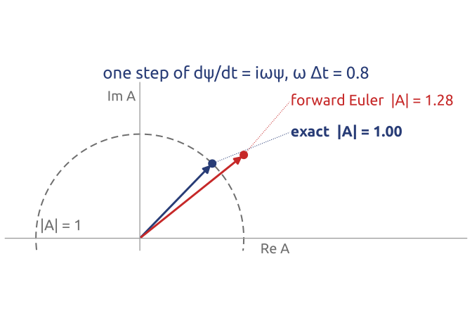
Forward Euler is unconditionally unstable for waves

(Durran 2010, sec. 2.2; Cushman-Roisin and Beckers 2011, sec. 2.6)

Ask first: forward Euler on a pure oscillation: does the amplitude grow, decay or stay? (It grows: the tangent step leaves the circle.) The angle is also wrong: arctan(w dt) < w dt.

Amplification (2/3): backward, trapezoidal

Backward Euler, the slope at the end (implicit):

\[\begin{aligned}&\psi^{n+1} = \psi^n + \Delta t\,(i\omega\psi^{n+1})\\ &\Rightarrow\; A = \frac{1}{1 - i\omega\Delta t}, \quad {\color{#1f5ccc}|A| < 1}\end{aligned}\]

Trapezoidal (Crank–Nicolson), the average of both:

\[\begin{aligned}&\psi^{n+1} = \psi^n + \frac{\Delta t}{2}\,i\omega\,(\psi^n + \psi^{n+1})\\ &\Rightarrow\; A = \frac{1 + i\omega\Delta t/2}{1 - i\omega\Delta t/2}, \quad {\color{#1f5ccc}|A| = 1}\end{aligned}\]

Damped, or neutral but slow; both implicit: a system to solve each step

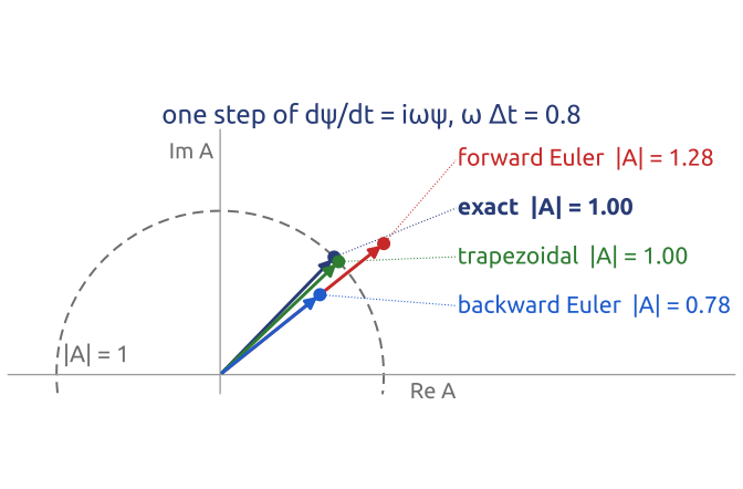
Implicit schemes are stable for any \(\Delta t\), at the price of a linear system per step

(Durran 2010, sec. 2.2.3)

Trapezoidal: neutral and second order, the phase lags: angle 2 arctan(w dt/2) < w dt. Semi-implicit models (IFS, lecture 7) use it for the gravity waves.

Amplification (3/3): leapfrog’s two roots

Leapfrog (Richardson’s step-over), centred in time:

\[\psi^{n+1} = \psi^{n-1} + 2\Delta t\,(i\omega\psi^n)\]

Try \(\psi^n = A^n\psi^0\): two roots,

\[\begin{gathered}A^2 - 2i\omega\Delta t\,A - 1 = 0\\ \Rightarrow\; A = i\omega\Delta t \pm \sqrt{1 - \omega^2\Delta t^2}\end{gathered}\]

• \(|\omega\Delta t| < 1\): both \(|A| = 1\), neutral (at \(1\) the two roots coincide)
• The root near \(-1\) is a computational mode: a zigzag of period \(2\Delta t\)

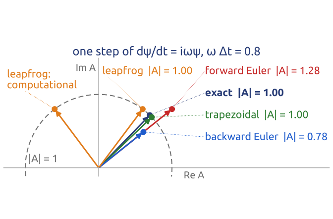
Leapfrog: explicit, neutral, second order, but with a spurious second solution

(Durran 2010, sec. 2.4; Lynch 1999)

Two time levels, so two solutions; the physical one tends to exp(i w dt). |w dt| > 1: one root grows, unstable. Two-level schemes have one root: no computational mode.

The inertial oscillation with four schemes

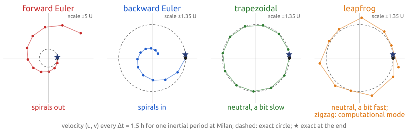
Step \(\Delta t = 1.5\) h at Milan (\(f\Delta t = 0.56\)): the velocity should go once round the circle

Same equation, same step: the scheme decides whether the current grows, dies or keeps its size

(Cushman-Roisin and Beckers 2011, secs. 2.6–2.9; Durran 2010, sec. 2.2)

After 11 steps: Euler x4.5, backward x0.22, trapezoidal x1 (2.5% slow per step), leapfrog 6% fast, its physical mode 10% too large and a 10% zigzag (computational mode), both from the first Euler step. Next: how to tame the zigzag.

Leapfrog’s zigzag and the Robert–Asselin filter

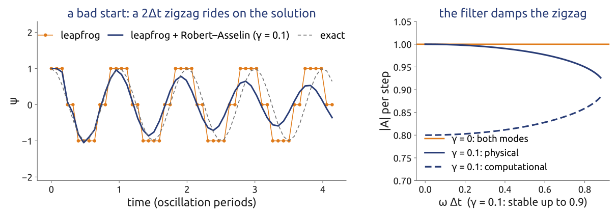
• After each leapfrog step, smooth in time: \(\;\bar\psi^n = \psi^n + \gamma\,(\bar\psi^{n-1} - 2\psi^n + \psi^{n+1})\), with the filter coefficient \(\gamma \approx 0.06\)–\(0.2\)
• It damps the zigzag fast (\(\times(1 - 2\gamma)\) per step), the physical mode slowly (here, with \(\omega\Delta t = 0.5\), by half in four periods): the scheme becomes first order

Leapfrog + Robert–Asselin ran most weather and climate models for decades

(Robert 1966; Asselin 1972; Durran 2010, sec. 2.4.2)

gamma = 0.06 typical in global models (Durran). Many models now use Runge-Kutta (next).

Runge–Kutta schemes and stability regions

Runge–Kutta: several slopes (stages) within one step; one time level, so no computational mode. The RK3 of Wicker and Skamarock (2002), for \(d\psi/dt = F(\psi)\):

\[\psi^* = \psi^n + \tfrac{\Delta t}{3}F(\psi^n),\quad \psi^{**} = \psi^n + \tfrac{\Delta t}{2}F(\psi^*),\] \[\psi^{n+1} = \psi^n + \Delta t\,F(\psi^{**})\]

On \(F = \lambda\psi\), with \(z = \lambda\Delta t\): \(\;A_{\mathrm{RK3}} = 1 + z + \dfrac{z^2}{2} + \dfrac{z^3}{6}\) (RK4 adds \(z^4/24\))

• Stability region: the \(z\) where \(|A| \le 1\)
• Waves (imaginary axis): RK3 stable for \(|\omega\Delta t| \le \sqrt{3}\), RK4 for \(|\omega\Delta t| \le 2\sqrt{2}\); Euler and RK2 never. MPAS uses an RK3

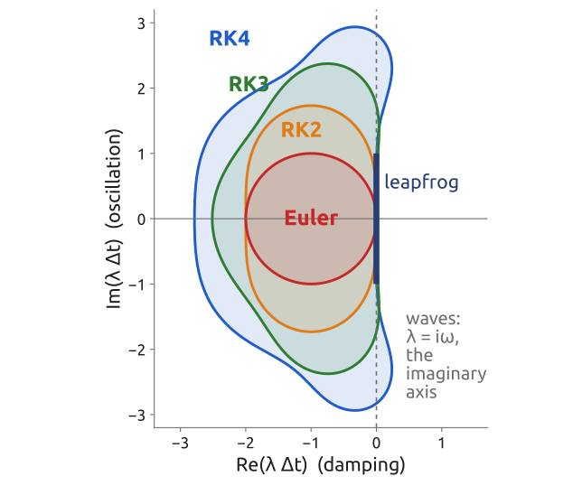
Explicit schemes for waves are stable only for \(|\omega\,\Delta t|\) below a limit of order one

(Durran 2010, sec. 2.3; Wicker and Skamarock 2002; Skamarock et al. 2012)

Each stage costs one evaluation of F: RK4 is four times Euler’s cost. The fastest wave sets the largest omega, hence the step: we will meet this as the CFL condition.

In class: forward Euler on the inertial oscillation

Exercise 1 — Forward Euler on the inertial oscillation. With \(w = u + iv\) the inertial oscillation \(du/dt = fv\), \(dv/dt = -fu\) is \(dw/dt = -ifw\). (a) One forward-Euler step multiplies \(w\) by a number \(A\): find \(A\) and \(|A|\). (b) At Milan (\(f = 1.04\times10^{-4}\,\mathrm{s^{-1}}\)) with \(\Delta t = 1\) h: by how much has the speed \(|w|\) grown after one inertial period, \(2\pi/f \approx 16.8\) h?

(c) To hand in: friction, and leapfrog. (i) Add a linear friction (drag) with rate \(r = 1/(1\ \text{day})\): \(dw/dt = -(if + r)\,w\). Find \(|A|\) for forward Euler. Can friction save it? For which \(\Delta t\) does the speed stop growing at Milan? (ii) Without friction, leapfrog: \(w^{n+1} = w^{n-1} - 2if\Delta t\,w^n\) (try \(w^n = A^n\)). What is the longest step at Milan that does not blow up? Which scheme would you use for the inertial currents of an ocean model, and why?

In notebook 05a (exercises 3 and 4): open in Colab · download

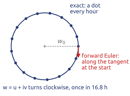
(Cushman-Roisin and Beckers 2011, secs. 2.6–2.7)

1. A = 1 - i f dt, |A| = sqrt(1 + (f dt)^2) = 1.068 for f dt = 0.374. (b) 16.8 steps: 1.068^16.8 = 3.0. (c)(i) A = 1 - (r + if)dt, |A|^2 = (1 - r dt)^2 + (f dt)^2 <= 1 iff dt <= 2r/(r^2 + f^2) = 2100 s (35 min); it then decays, but too slowly. (ii) A^2 + 2i f dt A - 1 = 0, |A| = 1 if f dt <= 1: dt <= 1/f = 2.7 h. Ocean: leapfrog (+ filter) or RK3; not Euler.

What the exercise showed

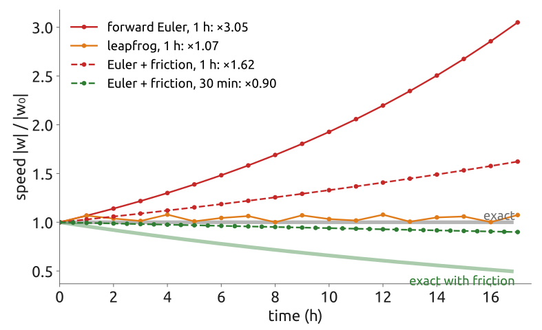
• Forward Euler: \(A = 1 - if\Delta t\), \(|A| = \sqrt{1 + (f\Delta t)^2} = 1.068\) with \(\Delta t = 1\) h: the speed triples in one inertial period
• Friction \(r = 1/(1\ \text{day})\): \(|A|^2 = (1 - r\Delta t)^2 + (f\Delta t)^2 \le 1\) only for \(\Delta t \le 2r/(r^2 + f^2) = 35\) min; even then it decays too slowly
• Leapfrog: \(|A| = 1\) for \(f\Delta t \le 1\): steps up to \(1/f = 2.7\) h at Milan
• For inertial currents: leapfrog (with a filter) or RK3, not Euler

Friction does not save forward Euler on waves; a neutral scheme does

(Cushman-Roisin and Beckers 2011, secs. 2.6–2.9; Durran 2010, sec. 2.2)

Leapfrog’s run shows a small zigzag: its first step is forward Euler (the computational mode).

Notebook Time stepping

Notebook 05a (open in Colab · download): time schemes on one ordinary differential equation, on a computer.

Stability regions of Euler and the Runge–Kutta schemes; leapfrog on the imaginary axis

1. From the equations to one ODE: the method of lines, the test equation
2. Euler’s method and its order: the error halves with \(\Delta t\)
3. Stability and the amplification factor 🧩 1
4. Stability regions and oscillations
5. Runge–Kutta 2, 3, 4: orders and stability regions 🧩 2
6. The inertial oscillation with six schemes ❗ 3 ❗ 4
7. The RK3 of MPAS (at home) 🧩 5

Predict, run, explain: write down what you expect before each run

One equation, many schemes: accuracy and stability measured on a computer

(Durran 2010, Ch. 2; Wicker and Skamarock 2002)

In class, 30 min: sections 2 to 6; section 7 at home. Adapted from Pedro’s 2023 MONAN course notebook 1. Walk round; stop at 10:45.

What the notebook showed

• Order: Euler’s error halves with \(\Delta t\); RK3 divides it by 8, RK4 by 16
• Stability is a separate question: on \(d\psi/dt = -60\psi\), Euler blows up for \(\Delta t > 1/30\) however accurate it is for small \(\Delta t\)
• Waves: only schemes whose stability region holds a piece of the imaginary axis survive (leapfrog, RK3, RK4, trapezoidal)
• Cost: stages are not free; the largest stable step per stage decides

But: so far time only. A whole field moving across the grid: how do space and time errors meet?

Accuracy (order) and stability (\(|A| \le 1\)) are different properties: check both

(Durran 2010, secs. 2.1–2.3)

Ask what they found for the largest RK4 step on the oscillation: omega dt = 2.83.

Advection: the simplest transport

A tracer \(q\) (humidity, salt) carried at constant speed \(c > 0\):

\[\frac{\partial q}{\partial t} + c\,\frac{\partial q}{\partial x} = 0, \qquad q(x,t) = q_0(x - ct)\]

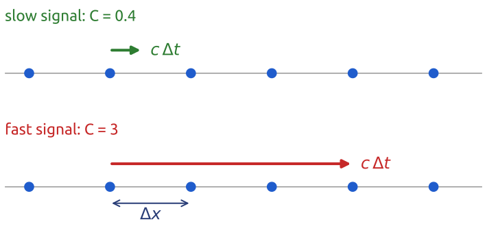
With the Courant number \(C = c\,\Delta t/\Delta x\):

• upwind: \(q_j^{n+1} = q_j^n - C\,(q_j^n - q_{j-1}^n)\)
• forward in time, centred in space (FTCS): \(q_j^{n+1} = q_j^n - \tfrac{C}{2}(q_{j+1}^n - q_{j-1}^n)\)
• leapfrog: \(q_j^{n+1} = q_j^{n-1} - C\,(q_{j+1}^n - q_{j-1}^n)\)
• Lax–Wendroff: FTCS \(+\,\tfrac{C^2}{2}(q_{j+1}^n - 2q_j^n + q_{j-1}^n)\)

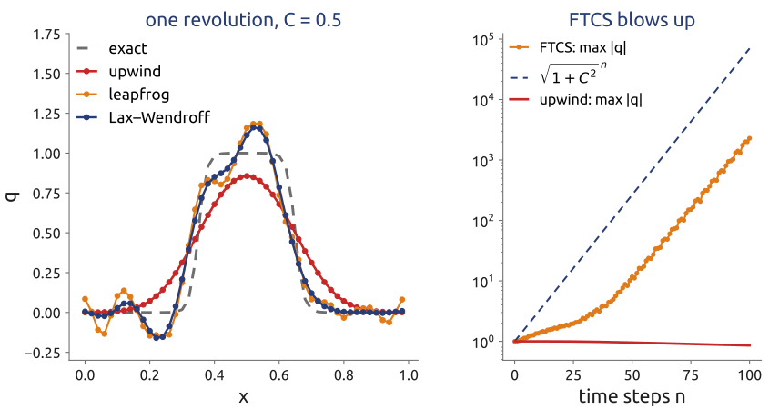
But: why does FTCS, centred and consistent, blow up?

Same equation, same step: smearing (upwind), wiggles (centred) or explosion (FTCS)

(Durran 2010, sec. 3.4; Lax and Wendroff 1960; FTCS: Kalnay 2003)

Upwind: take the difference on the side the flow comes from. Lax-Wendroff: Taylor in time, d2q/dt2 = c^2 d2q/dx2: second order. Left: one revolution, C = 0.5, 50 points.

Von Neumann (1/3): one Fourier mode at a time

On a periodic grid any field is a sum of modes \(e^{ikx}\), \(\;k\Delta x \in [-\pi, \pi]\). A linear scheme with constant coefficients only multiplies each mode:

\[q_j^n = A^n\,e^{\,i k j\Delta x}\]

\(k\): wavenumber; \(A\): amplification factor of the mode

Put it in the scheme, divide by \(A^n e^{ikj\Delta x}\): an equation for \(A(k\Delta x)\). Stable if \(|A| \le 1\) for every \(k\).

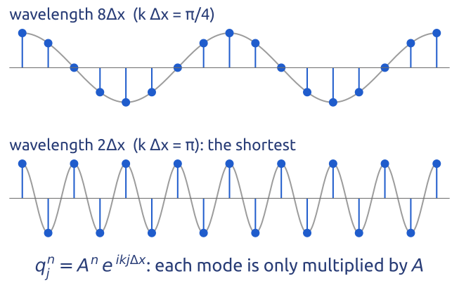
Von Neumann analysis: the amplification factor of each Fourier mode

(Durran 2010, sec. 3.2.2; Charney et al. 1950)

Charney et al. (1950, section V) used this Fourier analysis for the ENIAC forecast, “patterned after” Courant, Friedrichs and Lewy. The shortest mode is 2 dx: often the first to blow up.

Von Neumann (2/3): upwind is stable for \(C \le 1\)

Upwind, with \(\theta = k\Delta x\):

\[A\,e^{ikj\Delta x} = e^{ikj\Delta x} - C\left(e^{ikj\Delta x} - e^{ik(j-1)\Delta x}\right)\]

\[A = 1 - C + C\,e^{-i\theta}\]

• A circle of radius \(C\) centred at \(1 - C\)
• Inside the unit circle iff \(0 \le C \le 1\)
• \(C = 1\): \(A = e^{-i\theta}\), an exact shift by one cell

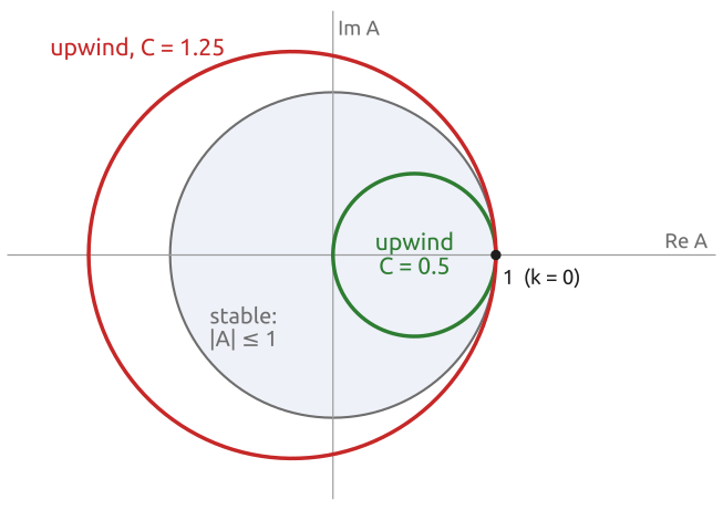
Upwind: stable if the flow crosses at most one cell per step, \(C = c\Delta t/\Delta x \le 1\)

(Durran 2010, sec. 3.2.2)

Ask first: upwind with C = 1, what happens? (q_j^{n+1} = q_{j-1}^n: the exact solution.) |A|^2 = 1 - 2C(1 - C)(1 - cos theta) on the board.

Von Neumann (3/3): FTCS is always unstable

FTCS, with \(\theta = k\Delta x\):

\[A = 1 - iC\sin\theta, \qquad {\color{#1f5ccc}|A|^2 = 1 + C^2\sin^2\theta > 1}\]

• A vertical segment through 1: outside for every \(C > 0\)
• Centred space gives imaginary eigenvalues, and forward Euler cannot take imaginary ones (the oscillation slides)
• Lax–Wendroff adds \(-C^2(1 - \cos\theta)\): back inside for \(C \le 1\)

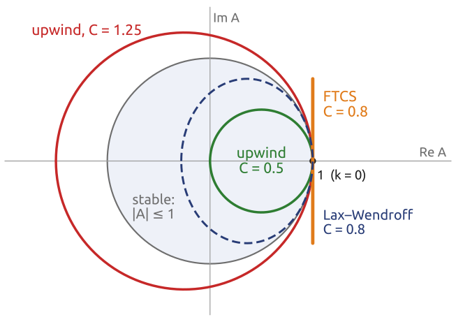
Consistent is not enough: FTCS approximates the equation and still blows up

(Durran 2010, secs. 3.2.2, 3.4.4)

Ask first: FTCS uses a centred, second-order difference and C = 0.5: is it stable? Worst mode theta = pi/2 (4 dx waves): growth sqrt(1 + C^2) per step, as in the run.

Eigenvalues on the stability regions

Method of lines: the space difference has eigenvalues \(\lambda(\theta)\); the scheme is stable if every \(\lambda\Delta t\) lies in the time scheme’s stability region.

• Upwind: \(\lambda\Delta t = -C(1 - e^{-i\theta})\), a circle: inside Euler’s disk if \(C \le 1\)
• Centred: \(\lambda\Delta t = -iC\sin\theta\), on the imaginary axis: never Euler; RK3 if \(C \le \sqrt{3}\); leapfrog if \(C \le 1\)

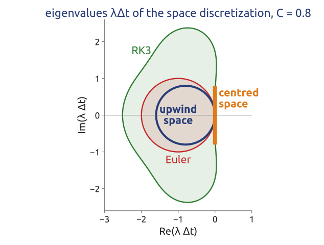
The time-stepping picture and von Neumann’s are the same picture

(Durran 2010, sec. 2.2.4)

Upwind space = damping (left half-plane); centred space = pure oscillation (imaginary axis). The fastest wave sets max |lambda| = c/dx (times sin): the limit is always on C.

Courant, Friedrichs and Lewy (1928)

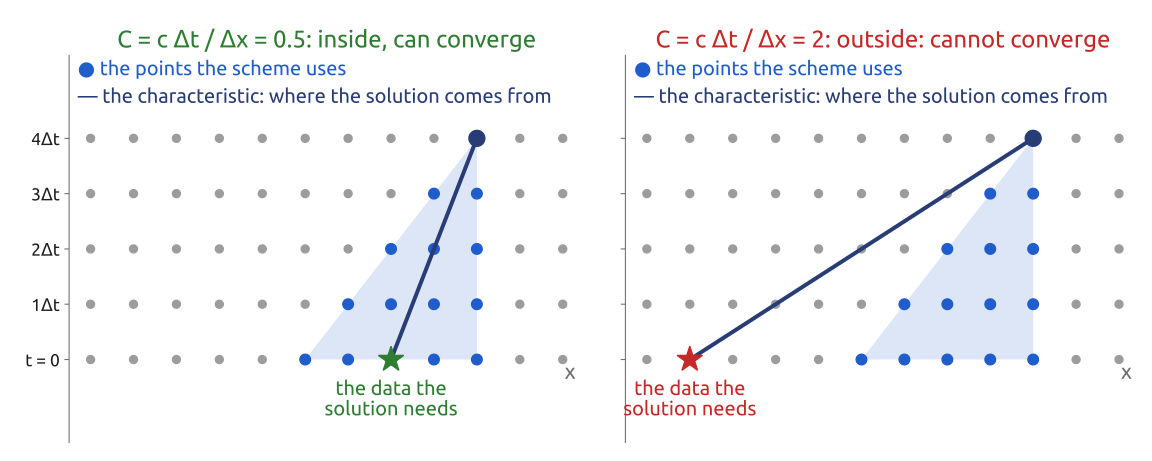
The solution at \((x_j, t^n)\) comes from \(x_j - ct^n\). An explicit scheme only sees the grid points in its stencil cone. If the true source lies outside, no choice of weights can converge.

CFL condition: the numerical domain of dependence must contain the true one (\(C \le 1\) here)

(Courant et al. 1928; Durran 2010, sec. 3.2.3; Lynch 2008)

Necessary, not sufficient: FTCS satisfies it and blows up. Courant, Friedrichs and Lewy wrote it for existence proofs, not computers; von Neumann knew it from Goettingen (Lynch 2008). Systems: c is the fastest wave speed.

Aside: the Lax–Richtmyer equivalence theorem

Theorem (Lax and Richtmyer 1956). For a well-posed linear initial-value problem and a consistent linear finite-difference scheme, stability is necessary and sufficient for convergence. A stable scheme accurate of order \((p, q)\) converges with error \(O(\Delta t^p) + O(\Delta x^q)\).

• Consistent: the truncation error \(\to 0\) as \(\Delta t, \Delta x \to 0\) (Taylor)
• Stable: \(\|q^n\| \le C_T\,\|q^0\|\) for \(n\Delta t \le T\), uniformly in \(\Delta t, \Delta x\)
• Consistency is the hypothesis, checked with Taylor; then stability, checked with von Neumann, is exactly what decides convergence

For a consistent scheme, stable \(\Leftrightarrow\) convergent: the reason we spend so long on \(|A|\)

(Lax and Richtmyer 1956; Durran 2010, sec. 3.2)

For the mathematicians. Consistency is a hypothesis, not a necessary condition: a scheme can converge without it (supraconvergence on non-uniform grids). Von Neumann’s |A| <= 1 is the stability test for constant coefficients on periodic grids; |A| <= 1 + O(dt) is allowed in general. Nonlinear problems: no such theorem.

Notebook Advection

Notebook 05b (open in Colab · download): advection in 1D, the CFL condition and von Neumann’s analysis, on a computer.

One revolution with \(C = 0.5\): upwind, leapfrog, Lax–Wendroff (left); FTCS blows up (right)

1. The problem: a bump carried round a periodic domain
2. Upwind with \(C = 1\), \(0.4\), \(1.2\)
3. The CFL condition: vary \(\Delta x\) and \(\Delta t\) ❗ 1 (why 1950 worked)
4. Six schemes side by side 🧩 2
5. Von Neumann: \(|A|\) measured on Fourier modes ❗ 3
6. Numerical diffusion and dispersion (at home)
7. Convergence (at home)

Predict, run, explain: which scheme keeps the height of the bump after one revolution?

Same equation, same step: the scheme decides between smearing, wiggles and explosion

(Durran 2010, secs. 3.2–3.4; Wicker and Skamarock 2002)

In class, 20 min: sections 2 to 5; 6 and 7 at home. Adapted from Pedro’s 2023 MONAN course notebook 2; the test profile is the one of Wicker and Skamarock (2002). Exercise 1 is the second in-class exercise (end of the lecture).

What the notebook showed: numerical diffusion

Taylor-expand the upwind scheme in \(\Delta t\) and \(\Delta x\): it solves, to second order, the modified equation

\[\frac{\partial q}{\partial t} + c\,\frac{\partial q}{\partial x} = {\color{#1f5ccc}\frac{c\,\Delta x}{2}\,(1 - C)}\,\frac{\partial^2 q}{\partial x^2}\]

• A diffusion we did not ask for: it smooths and lowers the bump
• It vanishes for \(C = 1\), and is negative (unstable) for \(C > 1\)

Centred schemes (leapfrog, Lax–Wendroff) keep the amplitude better but leave wiggles: their error term is a third derivative, \(\partial^3 q/\partial x^3\): dispersion, waves of different lengths moving at different speeds.

But: which waves are slow, and how slow?

Upwind smooths (numerical diffusion); centred schemes keep amplitude but disperse

(Durran 2010, secs. 3.3.2, 3.4.2)

Derivation on the board (notes): dq/dt + c dq/dx = (dx c/2) d2q/dx2 - (dt/2) d2q/dt2 + …, with d2q/dt2 = c^2 d2q/dx2 to this order (Durran, eq. 3.67). The diffusion coefficient for c = 10 m/s, dx = 100 km, C = 0.5: 2.5e5 m^2/s.

Phase speed: the \(2\Delta x\) wave stands still

Centred difference, a mode \(e^{i(kx - \omega t)}\):

\[\omega = \frac{c\,\sin(k\Delta x)}{\Delta x}, \qquad \frac{c^*}{c} = \frac{\sin(k\Delta x)}{k\Delta x}\]

\(c^* = \omega/k\): the phase speed on the grid; exact in time

• Long waves: right speed; short waves: too slow
• \(2\Delta x\): does not move (\(\omega = 0\))
• Group speed \(c\cos(k\Delta x) < 0\) for waves shorter than \(4\Delta x\): wiggles travel backwards, behind the bump
• Higher order helps, not at \(2\Delta x\)

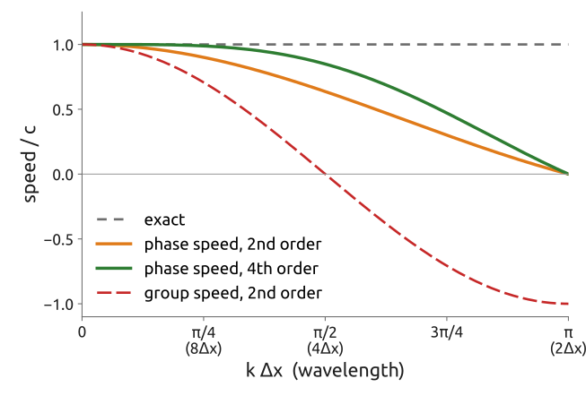
Grids are slow for short waves: resolve a feature with many points (8–10 per wavelength)

(Durran 2010, sec. 3.3.1; Randall 2011)

Semi-discrete (exact in time). Fourth order: (8 sin - sin 2theta)/(6 theta). Spectral methods (lecture 7) get the exact speed for every resolved wave.

A and C grids (1/2): where \(h\) and \(u\) live

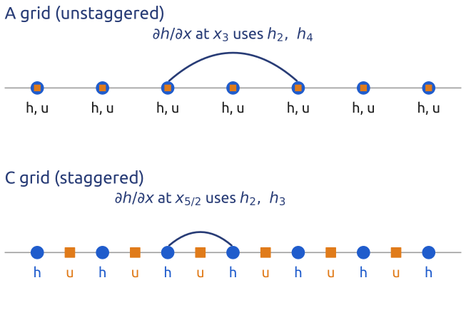
Linear gravity waves (height \(h = H + \eta\)): each equation needs the other variable’s derivative,

\[\partial_t h + H\,\partial_x u = 0, \qquad \partial_t u + g\,\partial_x h = 0\]

• A grid: \(h\) and \(u\) at the same points; centred differences over \(2\Delta x\)
• C grid (staggered): \(u\) half-way between the \(h\); differences over \(\Delta x\)
• Same number of unknowns per \(\Delta x\)

But: does it matter where they live?

Staggering puts each derivative where it is needed, at the shortest distance

(Mesinger and Arakawa 1976; Durran 2010, sec. 4.1.2)

Ask first: which grid lets a 2 dx wave of h move? Same number of unknowns per dx on both. The equations: lecture 3.

A and C grids (2/2): the \(2\Delta x\) mode

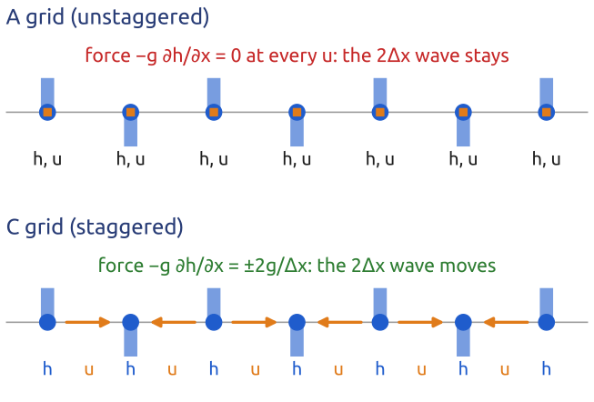
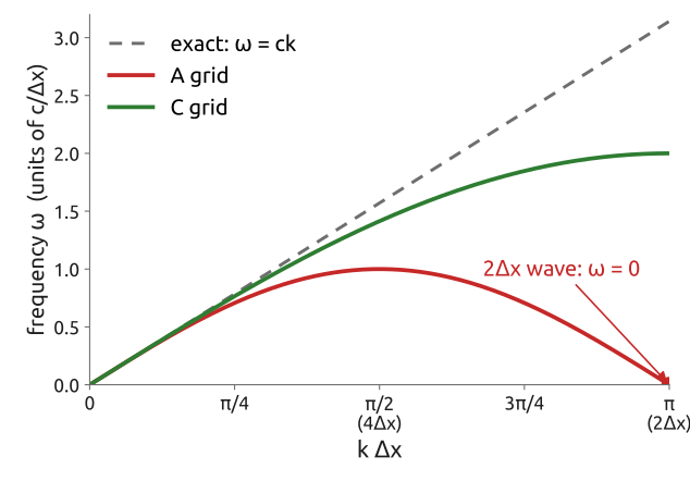
A: \(\omega = \dfrac{c}{\Delta x}\sin(k\Delta x)\) \(\quad\) C: \(\omega = \dfrac{2c}{\Delta x}\sin\dfrac{k\Delta x}{2}\)

A grid: the \(2\Delta x\) wave feels no force and stays, as noise; on the C grid it feels the largest

(Mesinger and Arakawa 1976; Randall 2011)

A checkerboard of h has zero centred gradient: no force on u, it stays (and accumulates noise). C grid: monotone omega, group speed > 0. Rotation adds a twist (lecture 6: A-E grids and L_d/dx). Leapfrog on the C grid needs c dt/dx <= 1/2 (max omega = 2c/dx).

The shallow water solver, opened

The solver behind the shallow water waves and the adjustment:

• Grid: C grid, \(\eta\) at cell centres, \(u\), \(v\) on the faces
• Space: centred differences over one \(\Delta x\); Coriolis by averaging
• Time: RK4, with \(\Delta t = 0.5\,\Delta x/c\), so \(C = 0.5\)

Is it stable? Fastest wave: the checkerboard, \(\omega_{\max} = 2c/\Delta x\) (1D), \(2\sqrt{2}\,c/\Delta x\) (2D). So \(\omega_{\max}\Delta t = 1\) and \(1.41\), inside RK4’s \(2\sqrt{2} = 2.83\): stable, with a margin of 2 to 3

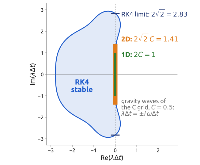
A grid, a difference, a time scheme and a step: each choice can now be checked on paper

(Durran 2010, secs. 2.2.4, 4.1.2; Randall 1994)

The solver of lecture 3’s notebook. Ask first: lecture 3 used RK4 with dt = 0.5 dx/c on the C grid. Could it double the step? (1D yes, up to C = sqrt 2; 2D only up to C = 1.) Rotation does not change the maximum: the averaged Coriolis term vanishes for the checkerboard. Energy: lost 0.2 % in 4 days, RK4’s |A| just below 1.

Notebook Shallow water in 1D

Notebook 05c (open in Colab · download): the shallow water solver opened, in 1D, to run, to test and to break.

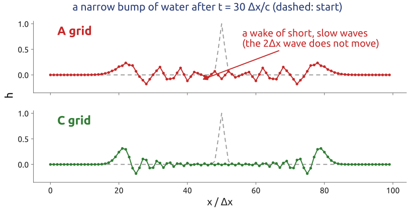
A narrow bump on the A grid (top) and the C grid (bottom)

1. The equations
2. The C grid
3. The RK3 of MPAS
4. A bump of water: geostrophic adjustment
5. Validation: geostrophic balance stays still
6. The time step (CFL): the largest stable \(\Delta t\) ❗ 1
7. A grid or C grid? What the A grid leaves behind
8. Mass

At home. Predict, run, explain: write down what you expect before each run

The black box in 1D: a grid, a difference, a time scheme and a step

(Wicker and Skamarock 2002; Randall 1994)

At home. Adapted from Pedro’s 2023 MONAN course notebook 3. Its exercise 1 (section 6, the largest stable time step) is mandatory. Lecture 6 starts from this C grid in 2D.

In class: why 1950 worked and 1922 did not

Exercise 2 — Why 1950 worked and 1922 did not. Compute the Courant number \(C = c\,\Delta t/\Delta x\) of Richardson’s forecast (grid about 200 km, leapfrog step \(\Delta t = 3\) h) and of the ENIAC forecast (\(\Delta x = 736\) km, \(\Delta t = 3\) h) for a wind of 20 m/s, a jet of 50 m/s and gravity waves at 300 m/s. Which signals could each scheme follow? Why could the ENIAC ignore the gravity waves?

(c) To hand in: an ocean model. A model with \(\Delta x = 10\) km over an ocean 4000 m deep: what is the longest explicit time step allowed by the surface gravity waves (\(c = \sqrt{gH}\), take \(C \le 1\))? And by currents of 1 m/s? How many steps per day does each need? What would you do?

In notebook 05b (exercise 1): open in Colab · download

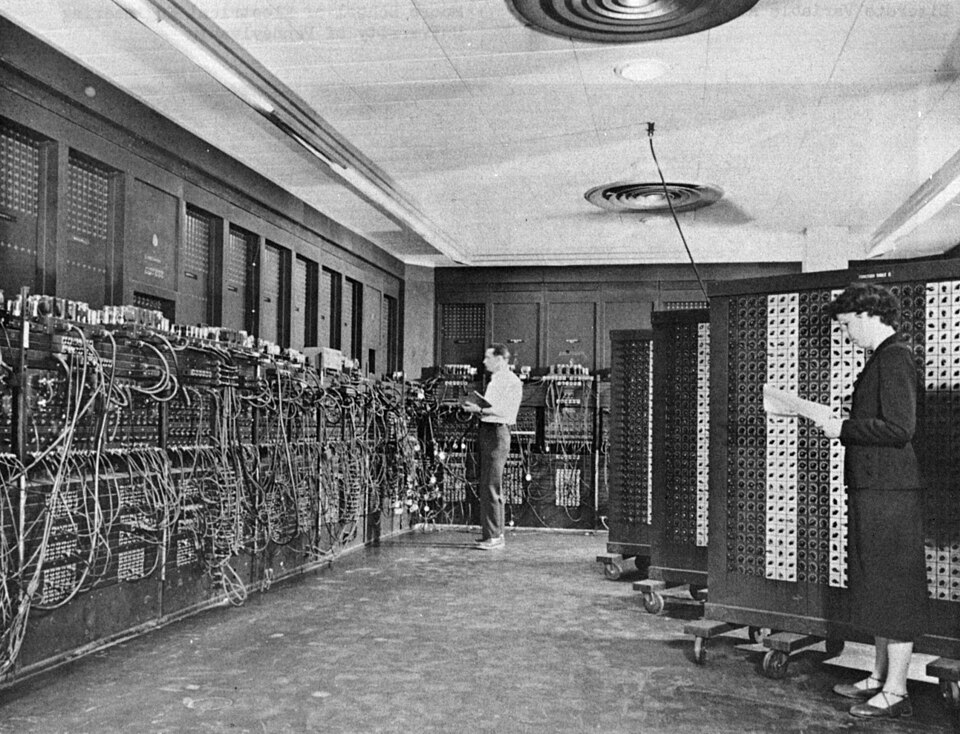
The ENIAC at Aberdeen. U.S. Army photo, public domain

(Lynch 1999; Charney et al. 1950) · Photo: commons.wikimedia.org: Glen Beck and Betty Snyder program the ENIAC

Richardson (200 km, 3 h): 1.1, 2.7, 16. ENIAC (736 km, 3 h): 0.29, 0.73, 4.4: fine for the winds; gravity waves are filtered out by the barotropic vorticity equation. Charney et al.: the primitive equations would need “some 15 minutes or less”. (c) sqrt(9.81*4000) = 198 m/s: 50 s, 1700 steps/day; currents: 10^4 s, 9 steps/day: split the fast mode (split-explicit) or implicit.

What the exercise showed

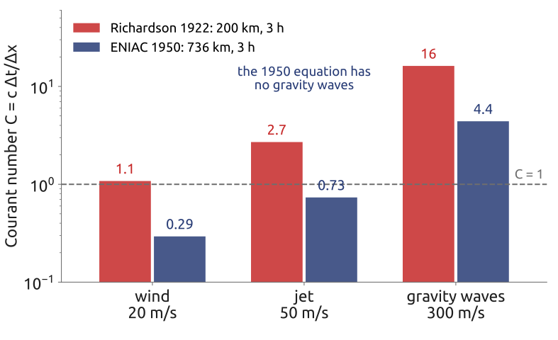
• Richardson (200 km, 3 h): \(C = 1.1\) for a wind, 2.7 for a jet, 16 for gravity waves: no explicit scheme can follow them
• The ENIAC (736 km, 3 h): 0.29 and 0.73 for the winds; the barotropic vorticity equation has no gravity waves, so their 4.4 never arises
• An ocean model, \(\Delta x = 10\) km, 4000 m deep: \(c = 198\) m/s gives \(\Delta t \le 50\) s, 1700 steps a day; currents of 1 m/s alone would allow \(10^4\) s, 9 steps a day: treat the fast waves apart (split-explicit, or implicit)

The fastest wave sets the explicit time step: filter it, split it, or treat it implicitly

(Lynch 1999; Charney et al. 1950)

Charney et al. (1950): the primitive equations would need “some 15 minutes or less”. Split-explicit and semi-implicit steps: lectures 7 and 9.

Key points

1. Order: a difference’s error falls like \(\Delta x^p\) (Taylor); centred differences: \(p = 2\)
2. Stability: \(|A| \le 1\) for every mode (von Neumann); forward Euler amplifies waves; leapfrog is neutral but has a computational mode; RK3/RK4 hold a piece of the imaginary axis
3. CFL: explicit schemes need \(C = c\,\Delta t/\Delta x \lesssim 1\): the fastest wave (gravity) sets \(\Delta t\). Necessary, not sufficient
4. Diffusion and dispersion: upwind smooths; centred schemes slow the short waves; the \(2\Delta x\) wave does not move
5. Staggering: on the C grid gravity waves have no \(2\Delta x\) null mode

Notebooks 05a (open in Colab · download), 05b (open in Colab · download) and 05c (open in Colab · download): exercise 1 comes back in 05a, exercise 2 in 05b.

Richardson’s method was the right one, his time step was not: the fastest wave sets \(\Delta t\)

Reading: (Durran 2010, Ch. 2–4; Cushman-Roisin and Beckers 2011, secs. 2.6–2.9; Döös et al. 2022)

Next lecture’s warm-up asks about these. Richardson: C about 16 for gravity waves; 1950: no gravity waves, so C < 1 with 3-h steps. Today’s models: C grids, Runge–Kutta or semi-implicit steps, the CFL number in every log file. Next: does a scheme keep the total mass? What about the wiggles that make negative humidity? And in 2D, with rotation, which grid? (lecture 6: finite volumes)