Finite volumes: conservation and the 2D shallow water equations
Atmosphere and Ocean Dynamics, Lecture 6: notes
Finite volumes: schemes that conserve mass, salt and heat exactly. These notes discuss cell averages updated by the fluxes through their faces; the donor cell and Godunov’s reconstruct–evolve–average view; flux limiters and Godunov’s theorem; the C grid as a finite-volume scheme in two dimensions, with the vector-invariant momentum equations; Arakawa’s grids A–E and their inertia–gravity waves; energy- and enstrophy-conserving averages (Sadourny); the M2 tide of an idealized Adriatic; and Voronoi meshes of the sphere, as in MPAS and MONAN.
1 Today’s goal: the tide of a closed sea
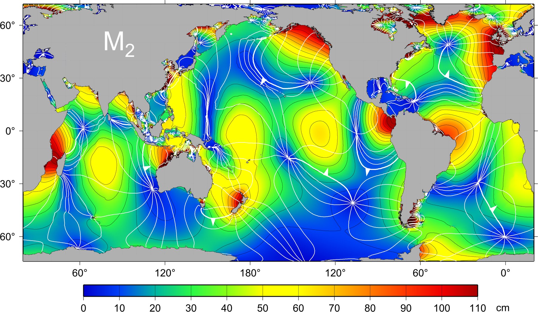
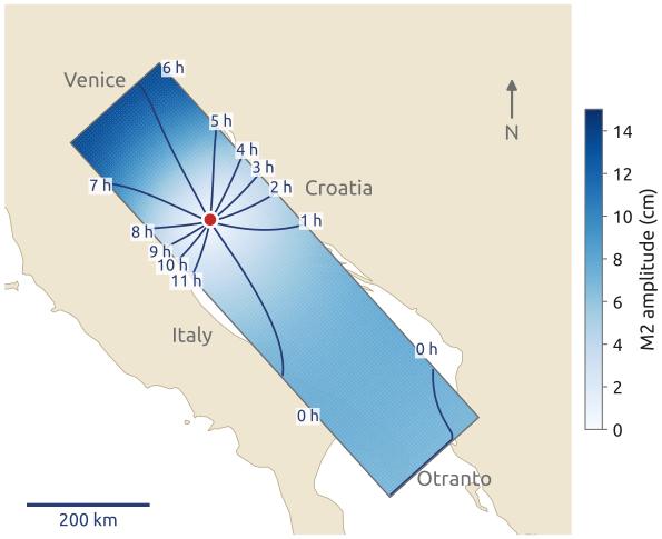
The slide shows the observed principal lunar tide, M2, from satellite altimetry (Figure 1), and the result to which the lecture leads: the M2 tide of an idealized Adriatic computed with Laplace’s tidal equations and friction (Figure 2). Tides are long waves on a rotating Earth; their lines of simultaneous high water turn around amphidromic points, where there is no tide. Two requirements come before such a computation. A model of a closed sea, or of the climate over centuries, must not create or lose water, salt or heat: a leak of 0.1% a day makes a model useless for climate. And the grid must represent the waves of a rotating fluid well: Kelvin waves, inertia–gravity waves, geostrophic adjustment. Finite volumes answer the first; the choice of a staggered grid, the second.
2 Finite volumes (1/3): a budget over a cell
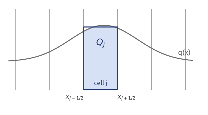
A control volume obeys a budget: the rate of change of what is inside equals what flows in minus what flows out. For a tracer \(q\) (a concentration) carried by a velocity \(c(x, t)\) in one dimension, with the flux \(F = c\,q\), over a cell \([x_{j-1/2}, x_{j+1/2}]\) of width \(\Delta x\) (Figure 3), \[ \frac{d}{dt}\int_{x_{j-1/2}}^{x_{j+1/2}} q\,dx = F(x_{j-1/2}, t) - F(x_{j+1/2}, t). \] If this holds for every interval and \(q\) is smooth, the integrand of \(\int(\partial_t q + \partial_x F)\,dx = 0\) must vanish: \(\partial_t q + \partial_x F = 0\), the conservation law in differential form. The integral form is the more fundamental one: it still makes sense where \(q\) jumps (a front, the edge of a plume), where derivatives do not; its solutions there are the weak solutions (LeVeque 2002, Ch. 2; Durran 2010, sec. 5.1).
3 Finite volumes (2/3): averages and fluxes
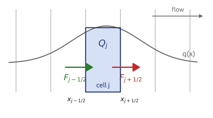
Dividing by \(\Delta x\) and calling \(Q_j(t) = \frac{1}{\Delta x}\int_{x_{j-1/2}}^{x_{j+1/2}} q\,dx\) the cell average, \[ \frac{dQ_j}{dt} = -\frac{F_{j+1/2} - F_{j-1/2}}{\Delta x}, \qquad F_{j\pm1/2} = F(x_{j\pm1/2}, t), \] still exactly. A finite-volume scheme takes the averages \(Q_j\) as the unknowns and makes one approximation: the numerical flux \(F_{j+1/2}\), computed from the averages of the cells near the face (LeVeque 2002, Ch. 4) (Figure 4). For many schemes on a uniform grid the formulas coincide with centred finite differences; the difference is in the interpretation (\(Q\) an average, \(F\) a flux), which matters on irregular meshes.
4 Finite volumes (3/3): the telescoping sum
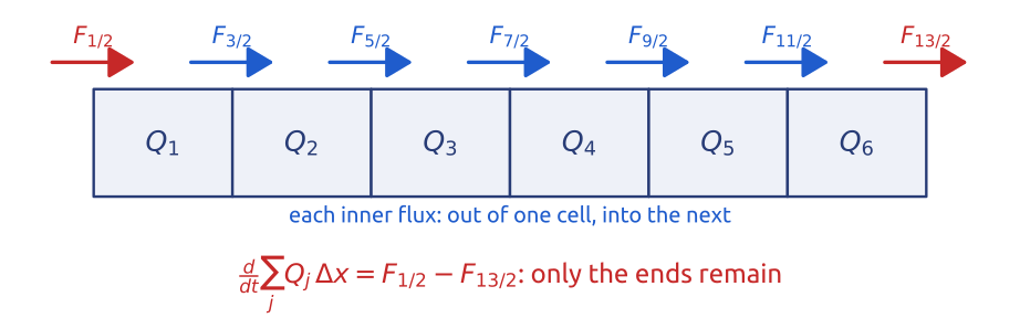
Sum over all cells: each inner flux \(F_{j+1/2}\) appears once with a minus sign (leaving cell \(j\)) and once with a plus sign (entering cell \(j+1\)), so \[ \frac{d}{dt}\sum_{j=1}^{n} Q_j\,\Delta x = F_{1/2} - F_{n+1/2}: \] a telescoping sum (Figure 5). The total changes only through the two ends; on a periodic domain or in a closed basin it does not change at all. This holds for any formula for the flux, any grid spacing (also non-uniform) and any time step, since the same telescoping applies to each step of an explicit scheme. Mass, salt, heat and tracers are conserved to round-off (LeVeque 2002, sec. 4.1; Durran 2010, sec. 5.2). A finite-difference discretization of the same equation in advective form, \(c\,\partial_x q + q\,\partial_x c\), is consistent but does not telescope: on a coarse grid its total drifts (Section 10).
5 Upwind is the donor cell
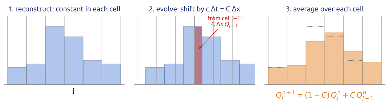
For a constant speed \(c > 0\) the simplest flux takes the value of the cell upstream, \(F_{j+1/2} = c\,Q_j\): \[ Q_j^{n+1} = Q_j^n - C\,(Q_j^n - Q_{j-1}^n), \qquad C = \frac{c\,\Delta t}{\Delta x}, \] the upwind scheme, now in conservation form: the donor-cell scheme. Godunov (1959) obtained it; in the reconstruct–evolve–average form of LeVeque (2002) (§4.10) it reads: take \(q\) constant in each cell (equal to \(Q_j\)), advance this staircase exactly by a distance \(c\,\Delta t \le \Delta x\), and average it again over each cell (Figure 6). The new average of cell \(j\) is \((1 - C)\,Q_j + C\,Q_{j-1}\): the part \(C\,\Delta x\,Q_{j-1}\) that crossed the left face is exactly the flux \(\Delta t\,F_{j-1/2}\); the cell upstream donates what crosses the face. For nonlinear systems, Godunov’s method solves a Riemann problem (the evolution of one jump) at every face (LeVeque 2002, secs. 4.9–4.11); for linear advection it reduces to upwind. The donor cell is monotone (each new value is a convex combination of old ones when \(C \le 1\), so no new extrema appear) and conservative, but first order and diffusive: it smears every front.
6 Higher order without new extrema: limiters
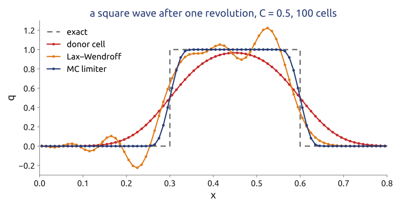
The Lax–Wendroff scheme in flux form is \[ F_{j+1/2} = c\left[\frac{Q_j + Q_{j+1}}{2} - \frac{C}{2}(Q_{j+1} - Q_j)\right] = c\,Q_j + \frac{c}{2}(1 - C)(Q_{j+1} - Q_j): \] the donor-cell flux plus a correction. It is second order but creates overshoots and undershoots near jumps (a negative concentration after one step, Section 9). A flux limiter multiplies the correction by a function \(\varphi(r_{j+1/2})\) of the ratio of successive jumps, \[ F_{j+1/2} = c\,Q_j + \varphi(r_{j+1/2})\,\frac{c}{2}(1 - C)(Q_{j+1} - Q_j), \qquad r_{j+1/2} = \frac{Q_j - Q_{j-1}}{Q_{j+1} - Q_j} \] (Durran 2010, sec. 5.5; LeVeque 2002, secs. 6.11–6.12). With \(\varphi = 0\) it is the donor cell, with \(\varphi = 1\) Lax–Wendroff. Where the solution is smooth, \(r \approx 1\) and the limiters keep \(\varphi \approx 1\) (second order); at an extremum \(r < 0\) and they set \(\varphi = 0\). Two classical choices: minmod, \(\varphi = \max(0, \min(1, r))\), and the monotonized centred (MC) limiter of van Leer (1977), \(\varphi = \max(0, \min(2r, (1 + r)/2, 2))\). Such schemes are total variation diminishing (TVD): the total variation \(\sum_j |Q_{j+1} - Q_j|\) never grows, so no new wiggles appear. They remain exactly conservative, since they only change the flux formula (Figure 7).
7 Mathematical aside: Godunov’s theorem
Theorem (Godunov 1959). A linear scheme for the advection equation that preserves monotonicity (never creates new extrema) is at most first-order accurate (Durran 2010, sec. 5.2). “Linear” means that the coefficients of the scheme do not depend on the solution, as for upwind, Lax–Wendroff or centred schemes of any order. High order without wiggles therefore requires nonlinear schemes: limiters (TVD), flux-corrected transport, ENO/WENO, the piecewise parabolic method. The price is that von Neumann’s analysis, which needs linearity, no longer applies directly. A related result of Harten: a TVD scheme is monotonicity preserving. Several operational models (MPAS among them) offer a monotonic transport option for tracers for this reason.
8 In class: one step by hand
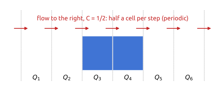
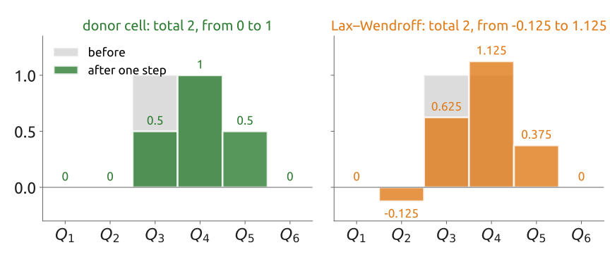
Exercise 1 — One step by hand. Six cells on a periodic line hold \(Q = (0, 0, 1, 1, 0, 0)\); the flow goes right with \(C = c\,\Delta t/\Delta x = 1/2\). (a) Do one step of the donor-cell scheme, \(F_{j+1/2} = c\,Q_j\). (b) Do one step of Lax–Wendroff, \(F_{j+1/2} = c\left[\tfrac12(Q_j + Q_{j+1}) - \tfrac{C}{2}(Q_{j+1} - Q_j)\right]\). (c) Compare the totals and the largest and smallest values with those of \(Q\).
(d) To hand in: an open channel. The same six cells, now a channel open at both ends: \(Q = (0, 0, 1, 1, 0, 0.5)\), a river brings in \(\Delta t\,F_{1/2}/\Delta x = 0.5\) through the left face, and water leaves through the right face with the donor-cell flux. Do one donor-cell step and show that the total changes by exactly \(\Delta t\,(F_{1/2} - F_{13/2})/\Delta x\), whatever happens inside.
9 What the exercise showed
With \(C = 1/2\) the donor-cell fluxes are \(\Delta t F_{j+1/2}/\Delta x = Q_j/2\), and one step gives \(Q = (0, 0, 0.5, 1, 0.5, 0)\); Lax–Wendroff gives \((0, -0.125, 0.625, 1.125, 0.375, 0)\) (Figure 9). Both keep the total, 2: the fluxes leave one cell and enter the next. The donor cell spreads the bump and stays between 0 and 1; Lax–Wendroff is sharper but makes a new minimum, \(-0.125\), and a new maximum, \(1.125\): Godunov’s theorem at work, for a linear second-order scheme. In the open channel of part (d) the scaled fluxes are 0.5 in through the left face, then 0, 0, 0.5, 0.5, 0 and 0.25 out through the right face: the new averages are \((0.5, 0, 0.5, 1, 0.5, 0.25)\) and the total goes from 2.5 to \(2.75 = 2.5 + 0.5 - 0.25\), exactly what came in minus what went out, whatever happens inside.
10 Finite volumes in 1D
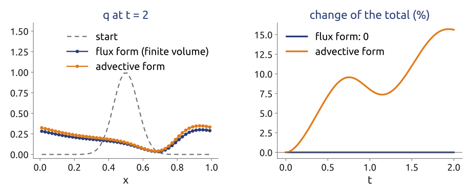
The computation of this part takes the steps of the lecture in turn: cell averages and fluxes; conservation by construction, comparing the flux form with the advective form of the same equation; the donor cell, with the exercise checked; limiters; and the fourth-order fluxes used, with a three-stage Runge–Kutta scheme, by the model MPAS (Wicker and Skamarock 2002). The test of conservation is a tracer carried by a speed that varies in space, \(c(x) = 1 + 0.5\sin 2\pi x\), on 50 cells (Figure 10): the flux form keeps the total to round-off, while the advective form, equally consistent and first order, drifts by 16% in two time units.
11 2D on the C grid: mass by fluxes
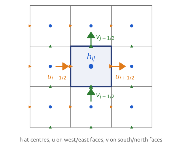
On a grid of square cells of side \(\Delta x\) the shallow water continuity equation \(\partial_t h + \nabla\cdot(h\mathbf{u}) = 0\), integrated over a cell, gives by the divergence theorem \[ \frac{dh_{ij}}{dt} = -\frac{(hu)_{i+1/2,j} - (hu)_{i-1/2,j}}{\Delta x} - \frac{(hv)_{i,j+1/2} - (hv)_{i,j-1/2}}{\Delta y}, \] with \(h_{ij}\) the mean depth of cell \((i, j)\) (\(i\) counts cells along \(x\), \(j\) along \(y\)) and the fluxes evaluated at the middle of each face (a second-order approximation of the face integral; in the nonlinear case the depth at a face is an average of the two cells beside it). The unknowns needed are the normal velocities on the faces: \(u\) on the west and east faces, \(v\) on the south and north faces. This is the staggered C grid, now read as a finite volume, and mass is conserved exactly by the same telescoping (Figure 11) (Sadourny 1975; Randall 2011). The momentum equations need more: \(v\) at the \(u\) points for the Coriolis term, and the vorticity.
12 2D on the C grid: momentum and vorticity
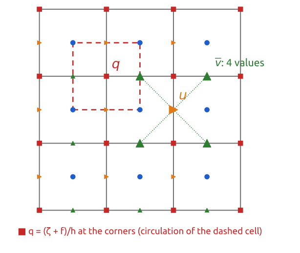
The momentum equations are easiest in vector-invariant form, \[ \frac{\partial\mathbf{u}}{\partial t} + q\,\mathbf{k}\times(h\mathbf{u}) = -\nabla B, \qquad q = \frac{\zeta + f}{h}, \quad B = gh + \tfrac12|\mathbf{u}|^2, \] with \(\zeta = \partial_x v - \partial_y u\) the relative vorticity, \(q\) the potential vorticity (from here on \(q\) is no longer a tracer) and \(B\) the Bernoulli potential. By Stokes’ theorem the vorticity averaged over a cell of the dual grid (the cell around a corner, joining the four neighbouring cell centres) is the circulation around it divided by its area: four velocities, one difference in each direction. So on the C grid the vorticity, and the potential vorticity, live at the corners. The pressure-gradient term \(-\partial_x B\) at a \(u\) face is a difference of the two cells beside it, with no averaging; the Coriolis–vorticity term at a \(u\) face needs \(v\), which lives on the other faces, and therefore an average of the four nearest \(v\) (Figure 12) (Sadourny 1975; Arakawa and Lamb 1977). Gravity waves need no averaging on the C grid; rotation does.
13 The Arakawa grids A–E
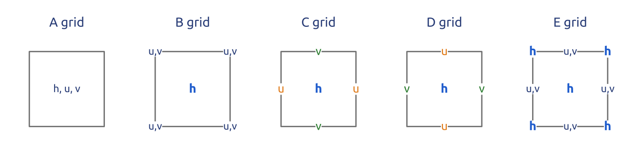
Arakawa and Lamb (1977) compared five ways to place \(h\), \(u\) and \(v\) on a square mesh, with the simplest centred differences on each (Figure 13): A (all at the cell centres), B (\(h\) at the centres, \(u\) and \(v\) together at the corners), C (\(u\) and \(v\) normal to the faces), D (\(u\) and \(v\) tangential to the faces) and E (a chequer-board of \(h\) and \((u, v)\), Richardson’s grid; see also Cushman-Roisin and Beckers (2011), §9.7). The A and B grids average the gravity-wave terms (for \(\partial h/\partial x\): A in \(x\), B in \(y\)); C averages only the Coriolis term; D averages almost everything. The E grid is a B grid turned by \(45^\circ\) (with the velocity components not turned), or equivalently two C grids shifted against each other; the A grid is four shifted C grids (Randall 2011). Where the unknowns live decides which terms are computed exactly and which need averages.
14 Inertia–gravity waves on the A, B, C grids
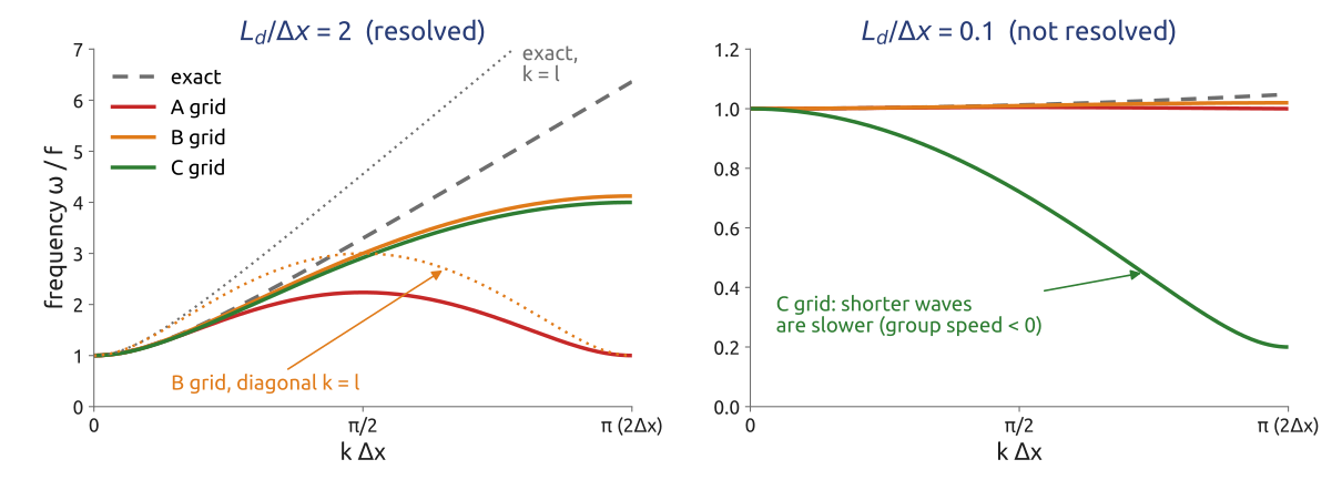
For the linearized shallow water equations on an \(f\)-plane, \(\partial_t h = -H(\partial_x u + \partial_y v)\), \(\partial_t u = fv - g\,\partial_x h\), \(\partial_t v = -fu - g\,\partial_y h\), with the simplest centred differences on each grid and continuous time, waves \(e^{i(kx + ly - \omega t)}\) have the frequencies (Randall 1994, 2011), with \(d\) the grid spacing and \(L_d = \sqrt{gH}/f\): \[ \begin{aligned} \text{exact:} &\quad (\omega/f)^2 = 1 + (L_d/d)^2\left[(kd)^2 + (ld)^2\right],\\ \text{A:} &\quad (\omega/f)^2 = 1 + (L_d/d)^2\left[\sin^2 kd + \sin^2 ld\right],\\ \text{B:} &\quad (\omega/f)^2 = 1 + 2(L_d/d)^2\left[1 - \cos kd\,\cos ld\right],\\ \text{C:} &\quad (\omega/f)^2 = \cos^2\tfrac{kd}{2}\cos^2\tfrac{ld}{2} + 4(L_d/d)^2\left[\sin^2\tfrac{kd}{2} + \sin^2\tfrac{ld}{2}\right]. \end{aligned} \] Figure 14 draws them for waves along \(x\); the figure script checks them against the eigenvalues of each scheme’s Fourier symbol. The exact frequency increases with the wavenumber, and so does the group speed: in geostrophic adjustment the energy of the unbalanced part is carried away by inertia–gravity waves, and a grid whose short waves have zero or negative group speed keeps that energy where it was, as noise.
- A grid: the gravity-wave terms need averages over \(2d\); \(\omega\) has a maximum at \(kd = \pi/2\) and returns to \(f\) at \(kd = \pi\): the short waves do not propagate. A-grid models are noisy and need filtering.
- B grid: the pressure gradient and the divergence need averages across the flow; along \(x\) the frequency is fine, but along the diagonal (\(k = l\)) it returns to \(f\) at \(kd = \pi\). Moderate problems, whatever \(L_d/d\).
- C grid: gravity waves need no averaging; only the Coriolis term does. When the deformation radius is resolved (\(L_d/d \gtrsim 1\); the figure uses 2) the frequency increases monotonically, close to the exact one. When it is not (\(L_d/d = 0.1\) in the figure) the averaged Coriolis term dominates and \(\omega\) decreases with \(k\): short inertia–gravity waves have the wrong group speed.
The conclusion of Arakawa and Lamb, and of Randall (1994): the C grid is the best choice when \(L_d/\Delta x \gtrsim 1\), the B grid copes better when the deformation radius is not resolved, which is why coarse ocean models (with \(L_d\) of tens of kilometres) long used the B grid. The same reasoning applies to each internal mode of a three-dimensional model, which has its own deformation radius. Randall (1994) also showed that an unstaggered grid for vorticity and divergence (his Z grid) behaves well for all \(L_d/\Delta x\).
15 In class: can the grid see the deformation radius?
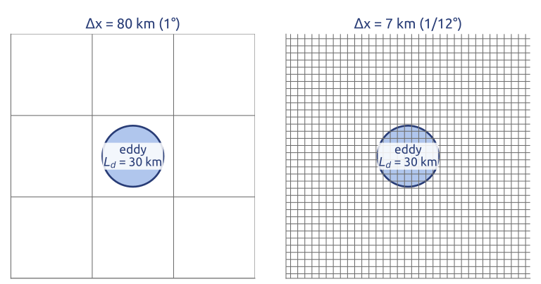
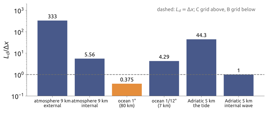
Exercise 2 — Can the grid see the deformation radius? Compute \(L_d/\Delta x\) and choose a grid (B or C) with the dispersion figure: (a) a global atmosphere model with \(\Delta x = 9\) km, external mode, \(L_d \approx 3000\) km; (b) the same model, a high internal mode with \(L_d \approx 50\) km; (c) ocean models with \(\Delta x = 80\) km (1°) and \(\Delta x = 7\) km (\(1/12^\circ\)), first baroclinic mode, \(L_d \approx 30\) km.
(d) To hand in: the Adriatic. A tide model of the Adriatic uses \(\Delta x = 5\) km at \(43^\circ\)N (\(f \approx 1.0\times10^{-4}\,\mathrm{s^{-1}}\)). Compute \(L_d = \sqrt{gH}/f\) for the tide in 50 m of water, and for an internal wave of speed 0.5 m/s. Is its C grid adequate for each?
16 What the exercise showed
The ratios are (Figure 16): (a) \(3000/9 = 330\) for the external mode of a 9 km atmosphere model, the C grid; (b) \(50/9 = 5.6\) for a high internal mode, still the C grid; (c) \(30/80 = 0.4\) for an ocean model of 1°, where the B grid copes better (as in many coarse ocean models), and \(30/7 = 4.3\) at \(1/12^\circ\), the C grid. (d) In the Adriatic, \(c = \sqrt{9.81\times50} = 22\) m/s and \(f = 1.0\times10^{-4}\ \mathrm{s^{-1}}\) give \(L_d = 220\) km, 44 cells of 5 km: well resolved. An internal wave of 0.5 m/s has \(L_d = 5\) km, one cell: poorly resolved; but a tide model of one layer has no internal waves. Eddy-resolving ocean models use the C grid for this reason.
17 Sadourny (1975): what the scheme conserves
With mass fluxes \(U = \overline{h}^x u\) and \(V = \overline{h}^y v\) on the faces, \(q\) at the corners and \(B = gh + K\), \(K = \tfrac12(\overline{u^2}^x + \overline{v^2}^y)\), at the centres (a bar with a superscript \(x\) is the average of two neighbours along \(x\), \(\delta_x\) their difference over \(\Delta x\)), Sadourny (1975) wrote \[ \frac{dh}{dt} = -\delta_x U - \delta_y V, \qquad \frac{du}{dt} = \overline{q\,\overline{V}^x}^{\,y} - \delta_x B, \qquad \frac{dv}{dt} = -\overline{q\,\overline{U}^y}^{\,x} - \delta_y B, \] and showed that this form of the Coriolis–vorticity term conserves the total energy \(\sum\left(\tfrac12 g h^2 + \tfrac12\overline{h}^x u^2 + \tfrac12\overline{h}^y v^2\right)\Delta x^2\) exactly in the semi-discrete equations; the alternative \(\overline{q}^{\,y}\,\overline{\overline{V}^x}^{\,y}\) (and its \(v\) counterpart) conserves the potential enstrophy \(\sum \tfrac12 \overline{h}^{xy} q^2\,\Delta x^2\) instead. Arakawa and Lamb (1981) found a scheme that conserves both. The motivation goes back to Arakawa’s work on the vorticity equation (Arakawa 1966): in two-dimensional flow, energy and enstrophy conservation constrain the transfer of energy between scales, and a scheme that respects them does not pile up energy at the grid scale over long integrations (nonlinear instability). The conservation is exact in space; the time scheme still breaks it a little (Figure 17).
18 Shallow water in 2D
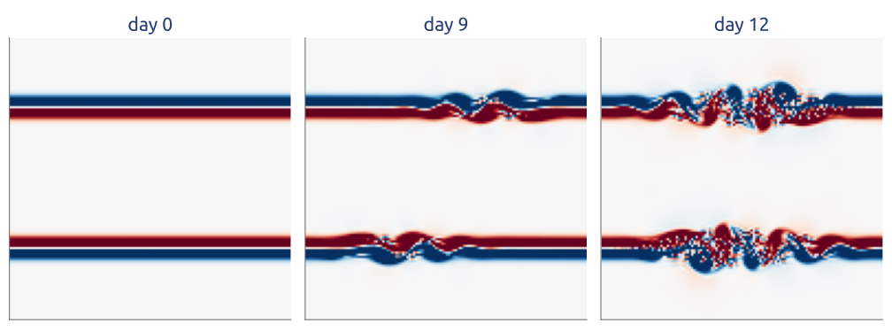
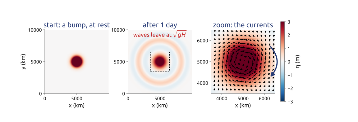
The two-dimensional computation follows the lecture: the C grid, Sadourny’s energy-conserving scheme, a three-stage Runge–Kutta step; a test with a steady geostrophic flow; the geostrophic adjustment of a Gaussian bump of water on an \(f\)-plane (\(H = 250\) m, \(f = 10^{-4}\ \mathrm{s^{-1}}\), \(L_d = 495\) km, cells of 100 km; Figure 18); the unstable jets of Figure 17; and the budgets of mass, energy and enstrophy. Around the bump the water turns clockwise, as the geostrophic wind does around a high pressure in the northern hemisphere.
19 What the notebook showed
A steady geostrophic flow drifts by \(O(\Delta x^2)\): the scheme is second order. In the adjustment, inertia–gravity waves leave at \(\sqrt{gH}\) and a balanced vortex stays; of a Gaussian bump of radius \(R\), about 17% of the excess volume stays for \(R = L_d/4\), 66% for \(R = L_d\) and 93% for \(R = 4L_d\) after one day: narrow bumps radiate, wide ones stay, as Rossby’s adjustment theory says (Randall 1994). Mass is conserved to round-off; energy up to the time-stepping error, which falls by a factor of about 6 when \(\Delta t\) is halved; the enstrophy error does not change with \(\Delta t\) (it comes from the space discretization). The enstrophy-conserving scheme shows the reverse. A real sea, though, has coasts and an open boundary.
20 Laplace’s tides in a closed basin
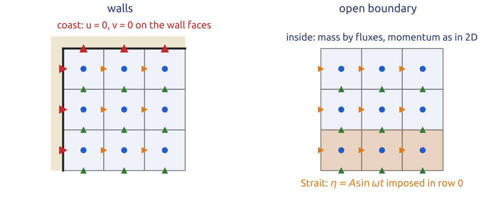
Laplace’s tidal equations, the linear shallow water equations, with a linear bottom friction of rate \(r\), \[ \frac{\partial\mathbf{u}}{\partial t} + f\,\mathbf{k}\times\mathbf{u} = -g\nabla\eta - r\,\mathbf{u}, \qquad \frac{\partial\eta}{\partial t} + \nabla\cdot(H\mathbf{u}) = 0, \] with \(\eta\) the sea level and \(H(y)\) the depth at rest, are solved on the C grid in a rectangle of \(200\times800\) km with walls on three sides and the Strait of Otranto open (the equilibrium-tide forcing is dropped; the tide enters at the Strait). On the C grid a coast is simply a face whose normal velocity is zero and never updated: no water crosses it, and mass is conserved exactly except through the Strait, where the sea level is imposed as the observed M2 tide, \(\eta = A\sin\omega t\) with \(A = 7\) cm (Janeković and Kuzmić 2005) (Figure 19). The depth increases from 35 m in the north to 400 m at the Strait (fitted so that the model’s seiche has about the observed period); constant \(f\) at \(43^\circ\)N, a friction with a decay time of 3.2 days, cells of 5 km, a fourth-order Runge–Kutta step. Cushman-Roisin and Beckers (2011), §9.8, discusses the numerical simulation of tides and storm surges; on an A grid the wall condition is much less natural.
21 The M2 tide of the Adriatic
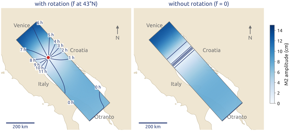
The computation of the tide first looks at the waves of the equations: gravity waves at \(c = \sqrt{gH}\) and Kelvin waves along the coasts, trapped within the deformation radius \(L_d = c/f\), about the width of the Adriatic (200 km against 190 km or more). It then builds the basin and the C-grid scheme, checks a Kelvin wave travelling along a wall, runs the M2 tide for 20 periods from rest and fits the last four by least squares: amplitude and phase in every cell, drawn as a cotidal chart (Figure 2). The tide enters at Otranto and travels north along the eastern (Croatian) coast, with the coast on its right: a Kelvin wave.
22 Rotation makes the amphidrome
The tide enters as a Kelvin wave travelling north along the Croatian coast, is reflected at the northern end and returns south along the Italian coast. The two waves make an amphidromic point, 252 km from the northern end in the model, around which high water turns anticlockwise, as observed. Venice has high water 6.6 h after Otranto (observed 6.4 h). Without rotation (\(f = 0\)) there is no amphidrome but a standing wave with a nodal line across the basin: the whole sea on each side rises together (Figure 20). The delays of high water at the tide gauges agree with the observations within about half an hour, while the amplitudes in the north are too small (13.5 cm at Venice against 23.4 cm observed): the real basin is closer to resonance at the M2 period (Janeković and Kuzmić 2005; Hendershott 1981).
23 Beyond rectangles: Voronoi grids
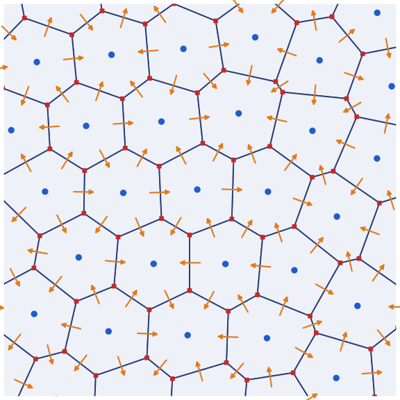
Latitude–longitude grids crowd their meridians at the poles, where the cells become very narrow and the CFL condition forces a tiny time step. Most new global models use quasi-uniform meshes of the sphere instead. The C grid generalizes to them: in MPAS (Skamarock et al. 2012) and in MONAN, the Brazilian model based on it, the mass lives in the cells of a Voronoi mesh, the velocity normal to each edge on the edges, and the vorticity at the vertices, the corners of the dual triangular mesh (Figure 21). The TRiSK scheme (Ringler et al. 2010) extends Sadourny’s ideas to such meshes: mass conserved by finite volumes, energy conserved, and potential vorticity dynamics consistent with the continuous equations.
24 Key points
- Conservation form: finite volumes update cell averages with face fluxes; the total changes only through the boundary: the reason ocean and climate models use them.
- Upwind = donor cell: first order, monotone, diffusive; higher order without new extrema needs a nonlinear limiter (Godunov’s theorem).
- Arakawa grids: the C grid (\(h\) in the cells, normal velocities on the faces) is right for gravity waves when \(L_d/\Delta x \gtrsim 1\); the B grid copes when it is not.
- Sadourny (1975): the C grid can conserve mass and energy, or mass and enstrophy; the same ideas on Voronoi grids make MPAS and MONAN.
- Tides: Laplace’s tidal equations with friction on the C grid give the M2 tide of the Adriatic, with its amphidrome.
Finite volumes keep mass by construction; on the C grid, energy or enstrophy too.
Further reading
LeVeque (2002) is the reference for finite volumes for hyperbolic problems; Durran (2010), Chapter 5, covers conservation laws, limiters and Godunov’s method with geophysical examples. Randall (2011) (course notes) discusses the grids A–E, the Z grid and other meshes; Mesinger and Arakawa (1976) and Arakawa and Lamb (1977) are the classics. Lauritzen et al. (2011) surveys the numerical methods of global atmospheric models, Vreugdenhil (1994) those of shallow-water flows in rivers, estuaries and coastal seas.