November 2026 · Politecnico di Milano

Finite volumes: conservation and the 2D shallow water equations

Atmosphere and Ocean Dynamics — Lecture 6

Prof. Dr. Pedro da Silva Peixoto

Applied Mathematics
Instituto de Matemática e Estatística
Universidade de São Paulo

Visiting Professor at MOX Lab
Politecnico di Milano

Warm-up

1. The centred difference \((q_{j+1} - q_{j-1})/(2\Delta x)\): what is its order, and how would you check it?
2. Forward Euler on \(d\psi/dt = i\omega\psi\): is \(|A|\) larger or smaller than 1? And leapfrog?
3. State the CFL condition for upwind advection. Is it enough for stability?
4. On which grid, A or C, does the \(2\Delta x\) gravity wave not move?

Lecture 5, from memory (2 minutes, then we discuss); its carry-forward list. Answers: Durran Ch. 2–4. Today: schemes that conserve by construction, and the grid for rotating waves in 2D.

1. Second order: halve dx, the error drops by 4 (log-log slope 2). 2. Euler sqrt(1 + w^2 dt^2) > 1; leapfrog |A| = 1 for |w dt| <= 1 (plus a computational mode). 3. C = c dt/dx <= 1; necessary, not sufficient (FTCS). 4. The A grid: the checkerboard has zero centred gradient.

Where we are and where we are going

Previous knowledge

• The centred difference is second order: halve \(\Delta x\), the error drops by 4
• Forward Euler amplifies waves, \(|A| = \sqrt{1 + \omega^2\Delta t^2} > 1\); leapfrog keeps \(|A| = 1\) for \(|\omega\Delta t| \le 1\) (with a computational mode)
• CFL for upwind: \(C = c\,\Delta t/\Delta x \le 1\); necessary, not sufficient (FTCS)
• On the A grid the \(2\Delta x\) gravity wave does not move; on the C grid it does
• A budget over a control volume: change inside = in − out (Gauss’s theorem)
• Shallow water: inertia–gravity waves \(\omega^2 = f^2 + gH(k^2 + l^2)\), \(L_d = \sqrt{gH}/f\); an unbalanced bump leaves a balanced vortex about \(L_d\) wide

Where we are going

1. Finite volumes: a budget over a cell
2. Donor cell, limiters; notebook in 1D
3. The C grid in 2D: mass and vorticity
4. The Arakawa grids against \(L_d/\Delta x\)
5. Sadourny’s scheme; notebook in 2D
6. Laplace’s tide in the Adriatic
7. Beyond rectangles: Voronoi grids

Build the conservation laws into the scheme, then choose the grid for rotating waves

(LeVeque 2002; Randall 1994)

Two minutes. Left: what we take as known (lectures 2, 3 and 5): the warm-up’s answers first. Right: the road of the day; each item links to its first slide.

Today’s goal: the tide of a closed sea

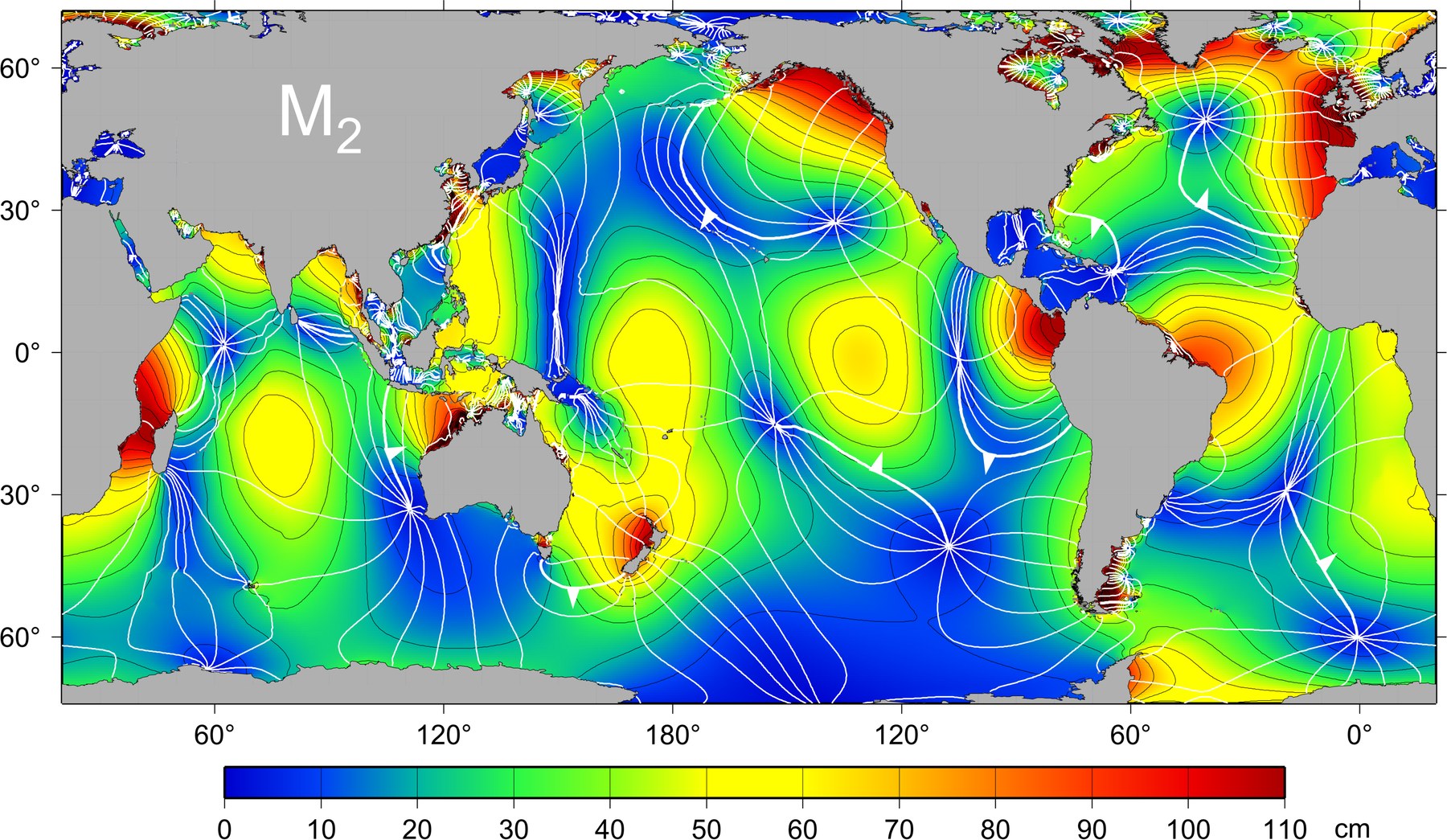
Observed M2 tide: R. Ray, NASA Goddard Space Flight Center, from TOPEX/Poseidon

• Tides are waves on a rotating Earth, with points of no tide (amphidromes)
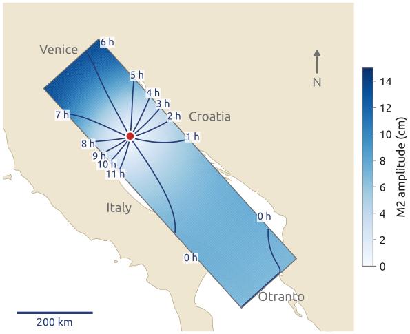
• By the end of today: Laplace’s tidal equations with friction in an idealized Adriatic:

But: a sea must not create or lose water; and which grid for rotating waves?

Conserve exactly what the sea holds, and get rotating gravity waves right

(Hendershott 1981) · Map: commons.wikimedia.org: M2_Tidal_constituent.tif

Callback to lecture 1: Newton’s tide, the amphidromic clock, Laplace (1776). The right panel is the result of the third notebook of today (amplitude in colour, hours of high water after Otranto as lines). A model that loses 0.1% of its water per day is useless for climate.

Finite volumes (1/3): a budget over a cell

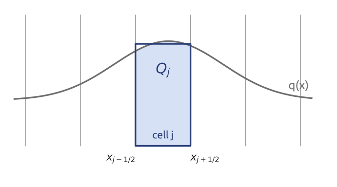
A control volume: the change of what is inside equals what flows in minus what flows out. For a tracer \(q\) with flux \(F = c\,q\), over the cell \([x_{j-1/2}, x_{j+1/2}]\):

\[\frac{d}{dt}\int_{x_{j-1/2}}^{x_{j+1/2}} q\,dx = F(x_{j-1/2}) - F(x_{j+1/2})\]

\(x_{j\pm1/2}\): the faces of cell \(j\); \(F\): the flux, here \(c\,q\)

For every cell, so (if \(q\) is smooth) \(\partial_t q + \partial_x F = 0\). Finite volumes keep the integral form.

Conservation laws are statements about volumes; derivatives come second

(LeVeque 2002, Ch. 2; Durran 2010, sec. 5.1)

Control volume: lecture 2. The integral form also holds for discontinuous q (fronts, the edge of a plume): the reason it is the fundamental one (weak solutions).

Finite volumes (2/3): averages and fluxes

Divide by \(\Delta x\); the unknown is the cell average \(Q_j = \frac{1}{\Delta x}\int_{\text{cell } j} q\,dx\):

\[\frac{dQ_j}{dt} = -\frac{{\color{#1f5ccc}F_{j+1/2}} - {\color{#1f5ccc}F_{j-1/2}}}{\Delta x}\]

\(Q_j\): cell average; \(F_{j\pm1/2}\): fluxes through its faces; \(\Delta x\): cell width

• Exact so far: no approximation yet
• The only approximation: the numerical flux \(F_{j+1/2}\) from the averages of the neighbouring cells

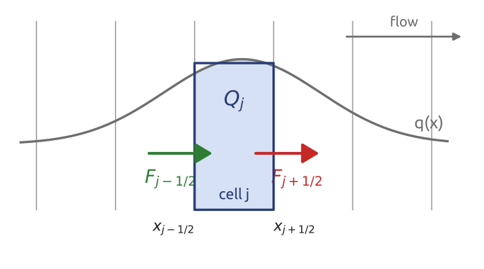
A finite-volume scheme is a recipe for the fluxes through the faces

(LeVeque 2002, Ch. 4)

Same equation as a centred finite difference in many cases; the difference is the interpretation: Q is an average, F a flux. On irregular meshes the difference matters (lecture 9).

Finite volumes (3/3): the telescoping sum

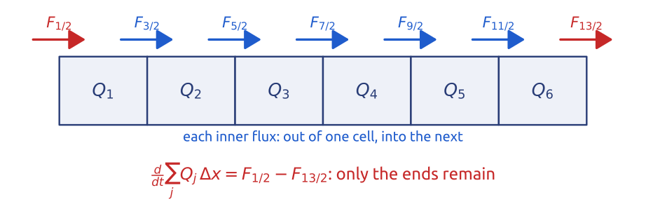
• Each inner face flux leaves one cell and enters the next: in \(\sum_j Q_j\,\Delta x\) the inner fluxes cancel in pairs
• The total changes only through the ends; on a periodic domain or a closed basin, not at all
• True for any flux formula, grid spacing or time step: conservation by construction

Finite volumes conserve mass (and salt, heat, tracers) exactly, up to round-off

(LeVeque 2002, sec. 4.1; Durran 2010, sec. 5.2)

Ask first: a finite-difference scheme for d(cq)/dx with variable c, written as c q_x + q c_x: does the total stay constant? (No: the notebook shows a 16% drift on a coarse grid.)

Upwind is the donor cell

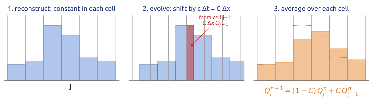
Godunov (1959), in LeVeque’s reconstruct, evolve, average form: reconstruct, evolve exactly, average. For \(c > 0\) the flux is \(F_{j+1/2} = c\,Q_j\): the cell upstream donates what crosses the face

The result is the upwind scheme, now conservative by construction

But: first order, and diffusive

Upwind = donor cell: monotone and conservative, but it smears every front

(Godunov 1959; LeVeque 2002, secs. 4.9–4.10)

Upwind: lecture 5. Godunov’s method for nonlinear systems solves a Riemann problem at every face; for linear advection it reduces to upwind. Higher order: reconstruct with slopes (MUSCL) or parabolas (PPM).

Higher order without new extrema: limiters

Lax–Wendroff flux = donor cell + a correction; a limiter \(\varphi(r)\) switches it off near jumps and extrema:

\[F_{j+1/2} = c\,Q_j + {\color{#1f5ccc}\varphi(r_{j+\frac12})}\,\frac{c}{2}(1 - C)(Q_{j+1} - Q_j)\]

\(C = c\,\Delta t/\Delta x\): Courant number; \(\varphi\): the limiter; \(r\): the ratio of successive jumps

• Smoothness at the face \(j+\tfrac12\): \(r_{j+\frac12} = \dfrac{Q_j - Q_{j-1}}{Q_{j+1} - Q_j}\) (\(\approx 1\) where smooth, \(< 0\) at an extremum)
• \(\varphi = 0\): donor cell; \(\varphi = 1\): Lax–Wendroff
• MC limiter: \(\varphi = \max\left(0, \min(2r, \tfrac{1+r}{2}, 2)\right)\)

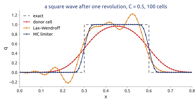
Limiters: second order where smooth, no new extrema near jumps, and still exactly conservative

(Durran 2010, sec. 5.5; LeVeque 2002, secs. 6.11–6.12; van Leer 1977)

Ask first: Lax-Wendroff is second order. On a square wave, better or worse than the donor cell? (Sharper, but overshoots to 1.22 and undershoots to -0.22: a negative humidity.) MC: van Leer (1977); the limiter idea: van Leer (1974).

Mathematical aside: Godunov’s theorem

Theorem (Godunov 1959). A linear scheme for the advection equation that never creates new extrema (monotonicity preserving) is at most first order accurate.

• Linear schemes: the coefficients do not depend on the solution (upwind, Lax–Wendroff, centred schemes of any order)
• So high order without wiggles needs a nonlinear scheme: limiters (TVD, FCT), ENO/WENO, PPM
• The price: the scheme is no longer linear, so von Neumann analysis no longer applies directly

Order and monotonicity: a linear scheme must choose one

(Godunov 1959; Durran 2010, sec. 5.2)

For the mathematicians. TVD: total variation does not grow; Harten’s theorem: TVD implies monotonicity preserving. MPAS has an optional monotonic transport for this reason.

In class: one step by hand

Exercise 1 — One step by hand. Six cells on a periodic line hold \(Q = (0, 0, 1, 1, 0, 0)\); the flow goes right with \(C = c\,\Delta t/\Delta x = 1/2\). (a) Do one step of the donor-cell scheme, \(F_{j+1/2} = c\,Q_j\). (b) Do one step of Lax–Wendroff, \(F_{j+1/2} = c\left[\tfrac12(Q_j + Q_{j+1}) - \tfrac{C}{2}(Q_{j+1} - Q_j)\right]\). (c) Compare the totals and the largest and smallest values with those of \(Q\).

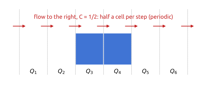
(d) To hand in: an open channel. The same six cells, now a channel open at both ends: \(Q = (0, 0, 1, 1, 0, 0.5)\), a river brings in \(\Delta t\,F_{1/2}/\Delta x = 0.5\) through the left face, and water leaves through the right face with the donor-cell flux. Do one donor-cell step and show that the total changes by exactly \(\Delta t\,(F_{1/2} - F_{13/2})/\Delta x\), whatever happens inside.

In notebook 06a (exercise 1): open in Colab · download

(LeVeque 2002, Ch. 4)

1. (0, 0, 0.5, 1, 0.5, 0). (b) (0, -0.125, 0.625, 1.125, 0.375, 0). (c) Totals 2 and 2; LW min -0.125, max 1.125. (d) Fluxes (dt/dx) F: 0.5 in, then 0, 0, 0.5, 0.5, 0, 0.25 out: new Q = (0.5, 0, 0.5, 1, 0.5, 0.25), total 2.75 = 2.5 + 0.5 - 0.25.

What the exercise showed

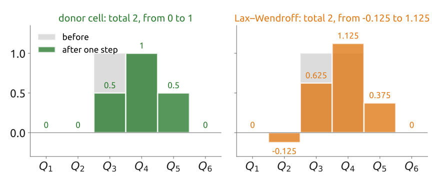
• Both keep the total, 2: the fluxes leave one cell and enter the next
• The donor cell spreads the bump and keeps it between 0 and 1; Lax–Wendroff is sharper but makes a new minimum (\(-0.125\)) and maximum (\(1.125\))
• Open channel: total \(2.5 \to 2.75 = 2.5 + 0.5 - 0.25\), exactly what came in minus what went out

Conservation is exact for any flux; monotonicity is not: that is the limiter’s job

(LeVeque 2002, Ch. 4; Durran 2010, sec. 5.2)

Lax-Wendroff’s new extrema are Godunov’s theorem at work: a linear second-order scheme cannot be monotone.

Notebook Finite volumes in 1D

Notebook 06a (open in Colab · download): fluxes, conservation and limiters in 1D, on a computer.

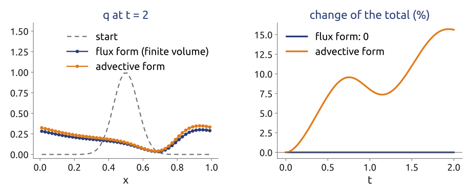
A speed that varies in space: the total, flux form against advective form

1. Conservation laws and cell averages
2. Conservation by construction: flux form against advective form
3. The donor cell: one step by hand ❗ 1
4. Limiters: higher order without new extrema ❗ 2 (at home)
5. The fourth-order fluxes of MPAS ❗ 3 (at home)

Predict, run, explain: which form keeps the total exactly?

Fluxes through faces: the total changes only through the boundary

(LeVeque 2002, Ch. 4–6; Wicker and Skamarock 2002)

In class, 15 min: sections 1 to 3; 4 and 5 at home (section 5 from Pedro’s 2023 MONAN notebook 2). Flux form: change 0 (round-off); advective form: +16% on 50 cells after two time units. Do not show the figure before they predict.

2D on the C grid: mass by fluxes

Shallow water: \(\partial_t h + \nabla\cdot(h\mathbf{u}) = 0\). Over a square cell, the divergence theorem:

\[\frac{dh_{ij}}{dt} = -\frac{(hu)_{i+\frac12,j} - (hu)_{i-\frac12,j}}{\Delta x} - \frac{(hv)_{i,j+\frac12} - (hv)_{i,j-\frac12}}{\Delta y}\]

• \(h\) at the centre, the normal velocities \(u\), \(v\) on the faces: the C grid, now a finite volume; \(i\) counts cells along \(x\), \(j\) along \(y\)

But: the momentum equations need \(v\) at \(u\) points (Coriolis), and vorticity

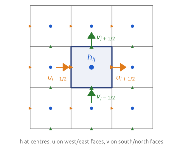
On the C grid, the mass equation is a finite-volume budget: water is conserved exactly

(Sadourny 1975; Randall 2011)

Shallow water: lecture 3; the 1D C grid: lecture 5. Flux on a face: the mid-face value times the face length (second order). The thickness h at the face is an average of the two cells (nonlinear case).

2D on the C grid: momentum and vorticity

Shallow water in vector-invariant form, with the potential vorticity \(q = (\zeta + f)/h\) (from here on \(q\) is the potential vorticity, not a tracer):

\[\frac{\partial \mathbf{u}}{\partial t} + q\,\mathbf{k}\times(h\mathbf{u}) = -\nabla\left(gh + \tfrac12|\mathbf{u}|^2\right)\]

\(\zeta\): relative vorticity; \(\mathbf k\): vertical unit vector; \(gh + |\mathbf u|^2/2\): the Bernoulli potential

• \(\zeta\) = circulation around the dual cell / its area: it lives at the corners
• Pressure gradient: a difference of the two cells beside a face, no averaging
• Coriolis term at a \(u\) point: an average of the four nearest \(v\)

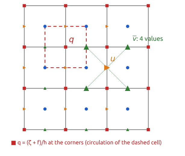
Gravity waves need no averaging on the C grid; rotation does. Is that a problem?

(Sadourny 1975; Arakawa and Lamb 1977)

PV: lecture 3. Kelvin’s circulation (lecture 1) on the grid: the vorticity of a dual cell is the sum of u.dl around it. That averaging of the Coriolis term is where the C grid can fail (next slides).

The Arakawa grids A–E

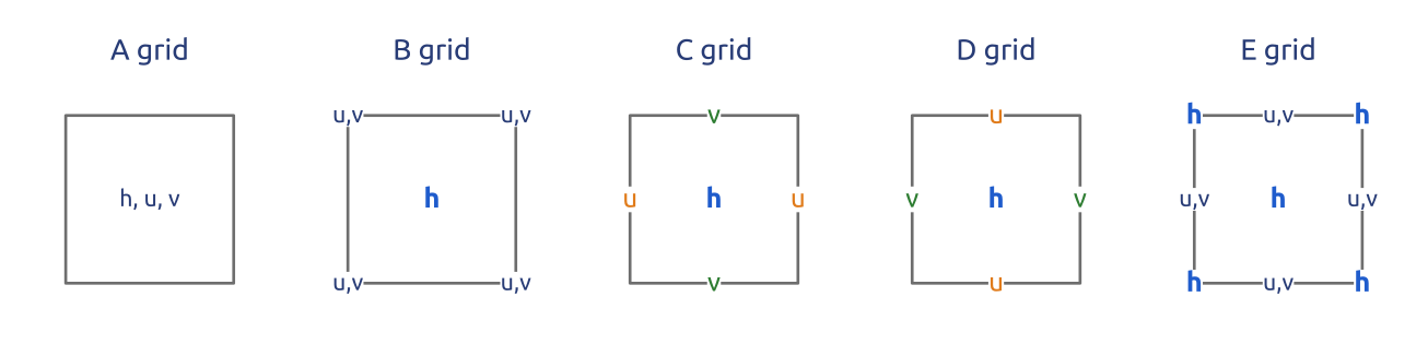
• Arakawa & Lamb (1977) compared five ways to place \(h\), \(u\), \(v\) for the linearized shallow water equations with rotation, with the simplest centred differences on each
• A and B average the gravity-wave terms (for \(\partial h/\partial x\): A in \(x\), B in \(y\)); C averages only the Coriolis term; D averages almost everything; E, Richardson’s chequer-board, is a B grid turned by 45°

Where the unknowns live decides which terms are computed exactly and which need averages

(Arakawa and Lamb 1977; Randall 2011; Cushman-Roisin and Beckers 2011, sec. 9.7)

Pure geometry; the question is how each grid represents geostrophic adjustment, that is, the inertia-gravity waves (next).

Inertia–gravity waves on the A, B, C grids

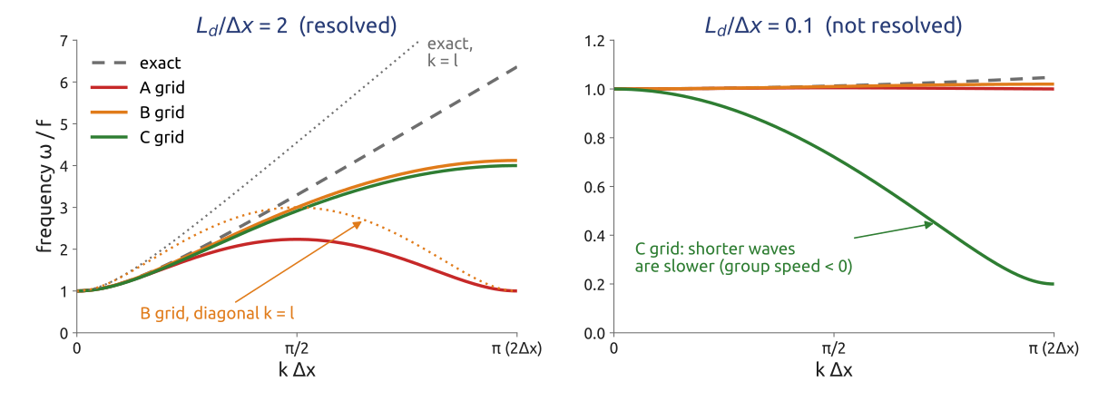
Exact: \(\omega^2 = f^2\left[1 + L_d^2(k^2 + l^2)\right]\), \(L_d = \sqrt{gH}/f\); each grid replaces \(k\) by a difference over \(\Delta x\) and averages some terms

C: excellent if \(L_d/\Delta x \gtrsim 1\), poor if not; B: fair in both cases; A: noisy when \(L_d\) is resolved

(Arakawa and Lamb 1977; Randall 1994)

Ask first: L_d/dx = 0.1 (deformation radius not resolved): does the C grid still propagate short inertia-gravity waves? (Badly: frequency falls with k, group speed reversed.) A grid: zero group speed at k dx = pi/2, as in lecture 5. L_d: lecture 3. B grid: fine along x, fails along the diagonal (dotted).

In class: can the grid see the deformation radius?

Exercise 2 — Can the grid see the deformation radius? Compute \(L_d/\Delta x\) and choose a grid (B or C) with the dispersion figure: (a) a global atmosphere model with \(\Delta x = 9\) km, external mode, \(L_d \approx 3000\) km; (b) the same model, a high internal mode with \(L_d \approx 50\) km; (c) ocean models with \(\Delta x = 80\) km (1°) and \(\Delta x = 7\) km (\(1/12^\circ\)), first baroclinic mode, \(L_d \approx 30\) km.

(d) To hand in: the Adriatic. A tide model of the Adriatic uses \(\Delta x = 5\) km at \(43^\circ\)N (\(f \approx 1.0\times10^{-4}\,\mathrm{s^{-1}}\)). Compute \(L_d = \sqrt{gH}/f\) for the tide in 50 m of water, and for an internal wave of speed 0.5 m/s. Is its C grid adequate for each?

In notebook 06c (exercise 1): open in Colab · download

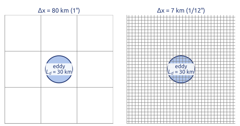
An eddy of radius \(L_d = 30\) km on two ocean grids, to scale

(Randall 1994; Arakawa and Lamb 1977)

1. 3000/9 = 330: C. (b) 50/9 = 5.6: C. (c) 30/80 = 0.4: B (as in many coarse ocean models); 30/7 = 4.3: C. (d) sqrt(9.81*50) = 22 m/s, f = 9.9e-5: L_d = 220 km, 44 cells: fine. Internal: 0.5/1e-4 = 5 km, one cell: poorly resolved, but the tide notebook has no internal waves.

What the exercise showed

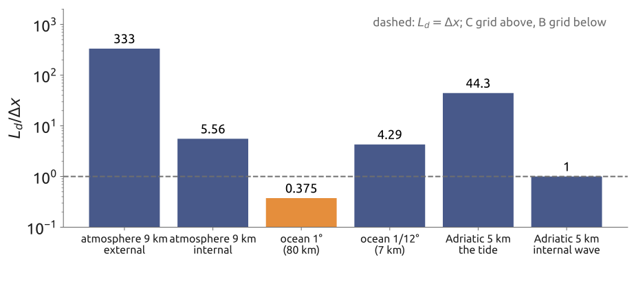
• The atmosphere resolves its deformation radii: \(L_d/\Delta x = 330\) and 5.6, the C grid
• The ocean at 1° does not (\(0.38\)): the B grid copes better; at 1/12° it does (4.3): the C grid
• The Adriatic tide: \(L_d = 220\) km, 44 cells; an internal wave of 0.5 m/s: 5 km, one cell, poorly resolved

The ratio \(L_d/\Delta x\) chooses the grid: the C grid where the deformation radius is resolved

(Randall 1994; Arakawa and Lamb 1977)

Coarse ocean models used the B grid for this reason (MOM up to version 4); eddy-resolving ones use the C grid.

Sadourny (1975): what the scheme conserves

Mass fluxes \(U = \overline{h}^x u\), \(V = \overline{h}^y v\) on the faces, \(q\) at the corners, \(B = gh + K\) at the centres:

\[\begin{aligned} \frac{du}{dt} &= {\color{#1f5ccc}\overline{q\,\overline{V}^x}^{\,y}} - \delta_x B\\ \frac{dv}{dt} &= -{\color{#1f5ccc}\overline{q\,\overline{U}^y}^{\,x}} - \delta_y B \end{aligned}\]

\(\overline{a}^x\): average of two neighbours along \(x\); \(\delta_x\): their difference over \(\Delta x\); \(K = |\mathbf u|^2/2\)

• This average conserves energy; another conserves potential enstrophy (Arakawa & Lamb 1981: both)
• Why: long runs keep the transfer between scales right, no pile-up at the grid scale

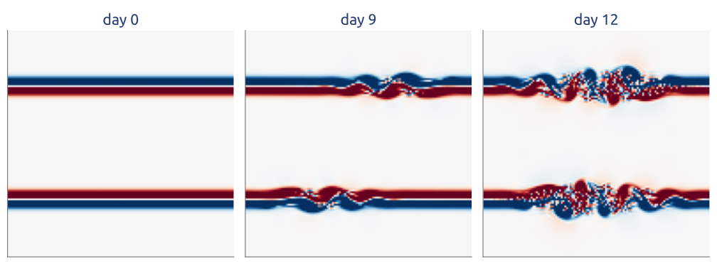
Two unstable jets roll up into vortices: vorticity, 128 × 128 cells (notebook, section 6)

Mimic the continuous invariants on the grid: mass exactly, and energy or enstrophy

(Sadourny 1975; Arakawa and Lamb 1977)

Arakawa (1966) did this for the vorticity equation (Jacobian). Exact in space; the time scheme still breaks it a little: in the notebook the energy error falls by about 6 when dt halves (RK3).

Notebook Shallow water in 2D

Notebook 06b (open in Colab · download): Sadourny’s scheme on the C grid in 2D, on a computer.

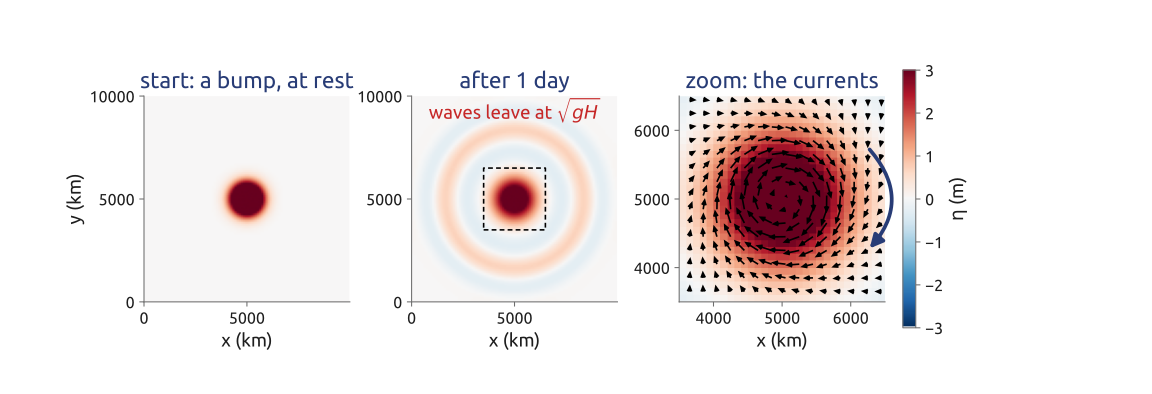
A bump of water adjusts: waves leave, a balanced vortex stays

1. The equations; 2. the C grid in 2D; 3. Sadourny’s scheme
2. Test: a steady geostrophic flow
3. Geostrophic adjustment of a bump ❗ 1
4. An unstable jet (at home)
5. What is conserved ❗ 2 (at home)

Predict, run, explain: which way does the water turn around the bump?

A shallow water model in a page of code, checked against geostrophy and Rossby’s adjustment

(Sadourny 1975; Peixoto and Schreiber 2019)

In class, 30 min: sections 2 to 5; 6 and 7 at home. Adapted from Pedro’s 2023 MONAN course notebook 4. f-plane, H = 250 m, L_d = 495 km, 100 km cells. Clockwise around a high in the north.

What the notebook showed

• Order: a steady geostrophic flow drifts by \(O(\Delta x^2)\)
• Adjustment: inertia–gravity waves leave at \(\sqrt{gH}\); a balanced vortex stays, with 17% of the water of a bump of radius \(L_d/4\), 66% for \(L_d\), 93% for \(4L_d\): narrow bumps radiate, wide ones stay
• Conservation: mass to round-off; energy up to the time-step error (÷ 6 when \(\Delta t\) halves); enstrophy not (or the reverse with the enstrophy-conserving scheme)

But: a real sea has coasts. How does a C grid handle walls, and an open boundary?

The model adjusts as Rossby’s theory says, and conserves what it was built to conserve

(Randall 1994; Sadourny 1975)

Numbers from the notebook runs (exercise 1, section 7). Rossby (1938): the adjustment problem (lecture 3).

Laplace’s tides in a closed basin

\[\begin{aligned} \frac{\partial \mathbf{u}}{\partial t} + f\,\mathbf{k}\times\mathbf{u} &= -g\nabla\eta - r\,\mathbf{u}\\ \frac{\partial \eta}{\partial t} + \nabla\cdot(H\mathbf{u}) &= 0 \end{aligned}\]

\(\eta\): sea level; \(H(y)\): depth at rest; \(r\): linear friction rate

• Walls: the normal velocity on a wall face is an unknown of the C grid: set it to zero
• Open boundary (Strait of Otranto): the sea level is imposed, \(\eta = A\sin\omega t\), M2
• Water is conserved exactly except through the Strait

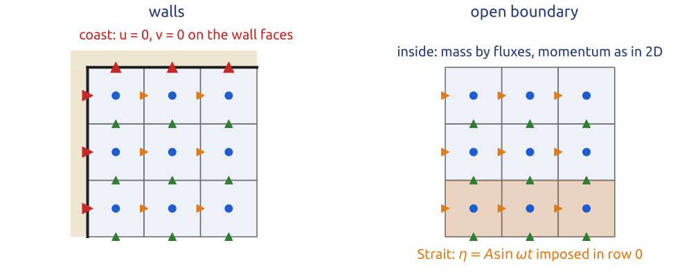
On the C grid, a coast is simply a face with zero flux

(Cushman-Roisin and Beckers 2011, sec. 9.8; Hendershott 1981)

Linear, constant f, friction r with a 3.2-day decay, depth 35 m in the north to 400 m at the Strait, 200 x 800 km, 5 km cells, RK4. On an A grid the wall condition is much less natural.

Notebook The M2 tide of the Adriatic

Notebook 06c (open in Colab · download): Laplace’s tidal equations on a C grid, in an idealized Adriatic.

The result to expect: M2 amplitude (colour) and hours of high water after Otranto (lines)

1. Motivation: the tide of Venice; 2. the equations
2. Waves first: \(c\), \(L_d = c/f\), Kelvin waves ❗ 1
3. The basin; 5. finite volumes on a C grid; 6. RK4 and the CFL limit
4. Validation: a Kelvin wave along a wall
5. The M2 tide: the cotidal chart; 9. model and observations
6. Exercises: no rotation ❗ 2; the seiche ❗ 3; resonance 🧩 4

Predict, run, explain: the tide enters at Otranto. Along which coast does it travel north?

A tide model of a sea in a page of code: walls are faces with zero flux

(Hendershott 1981; Janeković and Kuzmić 2005)

In class, 20 min: sections 3, 7, 8 and exercise 2; the rest at home. Along the eastern (Croatian) coast, with the coast on its right: a Kelvin wave. Back south along the Italian coast. Anticlockwise around the amphidrome, about 250 km from the northern end.

Rotation makes the amphidrome

• With rotation: Kelvin waves north along Croatia, south along Italy; high water turns anticlockwise around an amphidromic point (the amphidromic clock)
• Model: 252 km from the northern end, Venice 6.6 h after Otranto (observed 6.4 h)
• Without rotation: a standing wave with a nodal line across the basin
• Too small in the north (13.5 cm against 23 cm at Venice): the real basin is nearer resonance

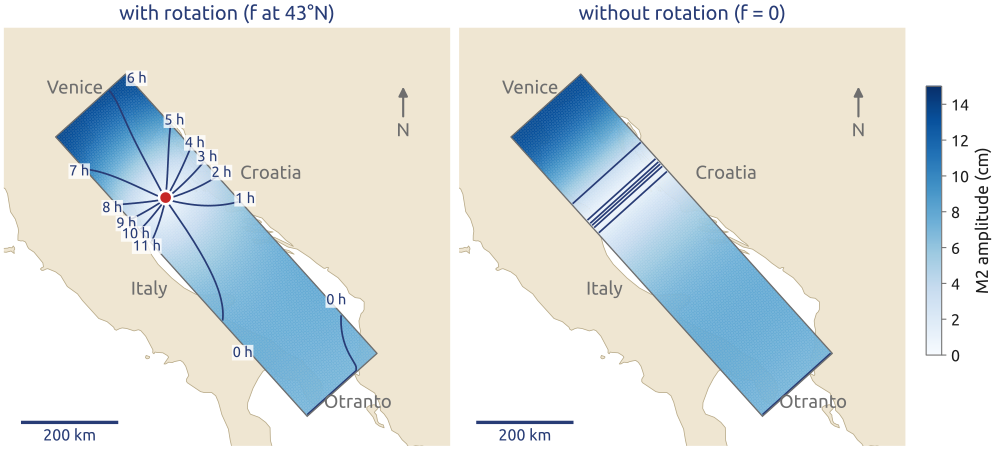
Laplace’s tidal equations (with friction) on a C grid of finite volumes: the amphidrome appears by itself

(Janeković and Kuzmić 2005; Hendershott 1981)

The clock: lecture 1. Ask first: with f = 0, is there still an amphidromic point? (No: a nodal line, the whole sea on each side rises together.) Delays and phases match the gauges well; amplitudes in the north ~40% low.

Beyond rectangles: Voronoi grids

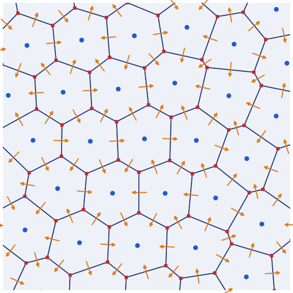
• Latitude–longitude grids crowd at the poles: tiny cells, tiny time steps (CFL)
• Quasi-uniform meshes of the sphere: cells of any shape; the C grid generalizes: \(h\) in the cells (●), normal velocities on the edges (→), vorticity at the vertices (■)
• TRiSK (Ringler et al. 2010): mass, energy and PV dynamics on any such C grid; used by MPAS (Skamarock et al. 2012) and MONAN

The ideas of today, cells, fluxes and a C grid, scale up to the sphere

(Ringler et al. 2010; Skamarock et al. 2012)

CFL: lecture 5. Pedro’s research: these grids and their errors. Lecture 9 shows the operational models (MPAS, ICON, FV3) and why they left the latitude-longitude grid.

Key points

1. Conservation form: finite volumes update cell averages with face fluxes; the total changes only through the boundary: the reason ocean and climate models use them
2. Upwind = donor cell: first order, monotone, diffusive; higher order without new extrema needs a nonlinear limiter (Godunov’s theorem)
3. Arakawa grids: the C grid (\(h\) in the cells, normal velocities on the faces) is right for gravity waves when \(L_d/\Delta x \gtrsim 1\); the B grid copes when it is not
4. Sadourny (1975): the C grid can conserve mass and energy, or mass and enstrophy; the same ideas on Voronoi grids make MPAS and MONAN
5. Tides: Laplace’s tidal equations with friction on the C grid give the M2 tide of the Adriatic, with its amphidrome

Notebooks 06a (open in Colab · download), 06b (open in Colab · download) and 06c (open in Colab · download): exercise 1 comes back in 06a, exercise 2 in 06c.

Finite volumes keep mass by construction; on the C grid, energy or enstrophy too

Reading: (Durran 2010, Ch. 5; LeVeque 2002; Randall 1994; Sadourny 1975)

Next lecture’s warm-up asks about these. Next: higher accuracy (spectral: lecture 7; finite elements: lecture 8); the sphere and the pole problem (lecture 9).