Spectral methods and the ECMWF model
Atmosphere and Ocean Dynamics, Lecture 7: notes
Spectral methods represent every field by global waves: Fourier series on a periodic interval, spherical harmonics on the sphere. These notes discuss the spectral derivative and its accuracy, products and aliasing (the transform method and the 2/3 rule), the barotropic vorticity equation on the sphere, semi-implicit time steps, the ECMWF model (IFS) and the cost of its transforms, the spectral models in use today, and the spectral method as a Galerkin method.
1 Two limits of grid methods
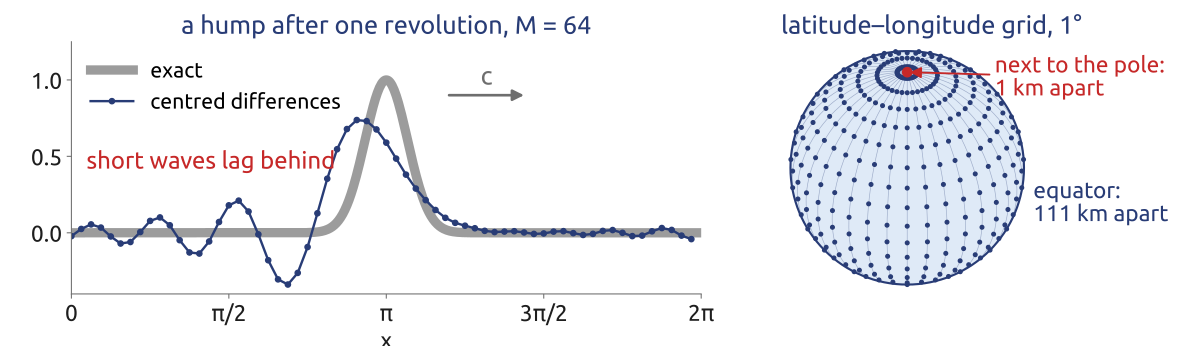
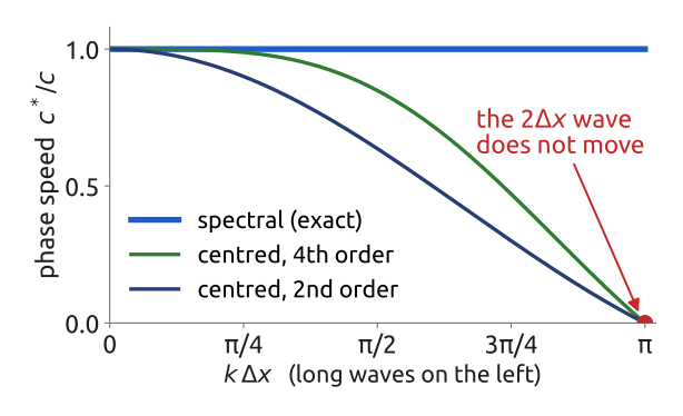
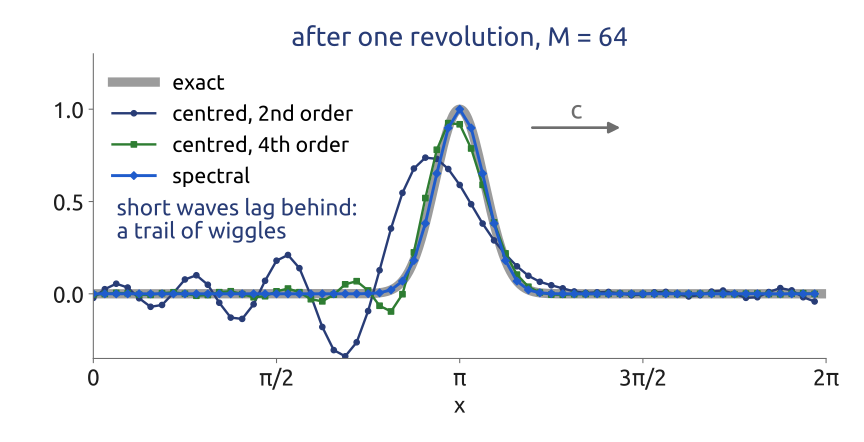
Grid-point methods have two limits (Figure 1). Applied to the advection of a wave \(e^{i(kx-\omega t)}\), the centred difference gives \(\omega = c\sin(k\Delta x)/\Delta x\), a phase speed \(c^* = \omega/k = c\sin(k\Delta x)/(k\Delta x) < c\): short waves move too slowly, and on \(M\) points the wave \(k = M/2\), of wavelength \(2\Delta x\), does not move at all; a narrow hump leaves a trail of wiggles behind it (numerical dispersion). On the sphere the CFL condition becomes the pole problem: on a latitude–longitude grid the meridians meet at the poles, and with a spacing of \(1^\circ\) the east–west distance between points is 111 km at the equator, 19 km at \(80^\circ\)N and 1 km on the row next to the pole (at \(89.5^\circ\)N, with the points at the centres of the cells). The CFL condition there forces a time step a hundred times shorter than at the equator, unless the short waves near the poles are filtered (Williamson 2007; Durran 2010, Sect. 3.3, 6.4.2). Can a derivative be exact for every wave the grid carries, and can a global model avoid the tiny steps of the poles?
2 Von Neumann’s trick (1950)
The ENIAC forecast of Charney et al. (1950) was a finite-difference model, and a regional one. The barotropic vorticity equation for the 500 hPa height was written on a polar stereographic map, a plane tangent at the North Pole; the curvature of the Earth then enters only through the map factor \(m = 2/(1 + \sin\varphi)\), with \(\nabla^2_{\text{globe}} = m^2\nabla^2_{\text{map}}\) and \(J_{\text{globe}} = m^2 J_{\text{map}}\), so that the operators are those of a flat plane. The domain was a rectangle over North America of 19 by 16 grid points (\(P = 18\) by \(Q = 15\) intervals \(\Delta s\), 736 km at the pole and 494 km at \(20^\circ\)N), with centred differences in space and a leapfrog step in time (Lynch 2008, appendix A). A regional domain needs boundary conditions: Charney, Fjørtoft and von Neumann showed that the height on the whole boundary, and the vorticity where the flow enters, determine the motion, and the boundary heights were held fixed through each 24-hour forecast.
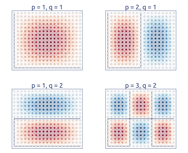
At every step the Jacobian gave the tendency of the vorticity, and the tendency of the height (here written with the streamfunction, \(\psi = gz/f_0\) in Lynch’s re-creation) followed from a Poisson problem, zero on the boundary: \[ (\delta_x^2 + \delta_y^2)\,\partial_t\psi = -J(\psi, \zeta + f), \qquad \delta_x^2 f_i = \frac{f_{i+1} - 2f_i + f_{i-1}}{\Delta s^2} , \] with the 5-point Laplacian \(\delta_x^2 + \delta_y^2\) built from centred second differences (notation of Durran 2010, Sect. 3.1) and the map factor on the right-hand side. Platzman (1979, 310) tells that, of the arithmetic done by the ENIAC, “the only nontrivial ones were the four in which the Laplacian was inverted to solve Poisson’s equation”. Von Neumann solved it with a direct method. With zero boundary values, the discrete sines are the eigenvectors of the 5-point Laplacian: from \(\sin(a + b) + \sin(a - b) = 2\sin a\cos b\), \[ \delta_x^2 \sin\frac{p\pi i}{P} = \frac{2\cos(p\pi/P) - 2}{\Delta s^2}\,\sin\frac{p\pi i}{P} = -\frac{4}{\Delta s^2}\sin^2\frac{p\pi}{2P}\,\sin\frac{p\pi i}{P} , \] and likewise in \(y\), so that \[ (\delta_x^2 + \delta_y^2)\Big[\sin\frac{p\pi i}{P}\,\sin\frac{q\pi j}{Q}\Big] = -\frac{4}{\Delta s^2}\Big[\sin^2\frac{p\pi}{2P} + \sin^2\frac{q\pi}{2Q}\Big]\,\sin\frac{p\pi i}{P}\,\sin\frac{q\pi j}{Q} , \] for \(p = 1, \dots, P - 1\) and \(q = 1, \dots, Q - 1\). Expanding the right-hand side in these sines (a sine transform in \(x\), then one in \(y\)), dividing each coefficient by its eigenvalue, and summing back (two more sine sums) gives the tendency: the four transforms of each step, Platzman’s operations 5, 8, 11 and 13. In his words, it is “one of a class of direct methods in which an exact solution of the discrete problem is obtained in a finite number of steps”, chosen because of the peculiar limitations of the ENIAC (Platzman 1979, 310; Lynch 2008, appendix A).
So the 1950 forecast was not a spectral model: the derivatives, the Jacobian included, were finite differences, and the sines only inverted the discrete Laplacian. The eigenvalue is the square of the modified wavenumber of the centred difference, \((2/\Delta s)\sin(p\pi/2P)\): for long waves it tends to the eigenvalue of the exact Laplacian on the rectangle, \(-[(p\pi/L_x)^2 + (q\pi/L_y)^2]\) with \(L_x = P\Delta s\), \(L_y = Q\Delta s\), and it is smaller for short ones. Spectral methods go further: they represent every field, and every derivative, by a sum of eigenfunctions of the exact Laplacian: on a periodic interval the Fourier waves, on the sphere the spherical harmonics. The first model of that kind was Silberman’s, in 1954 (Silberman 1954).
3 Global or local?
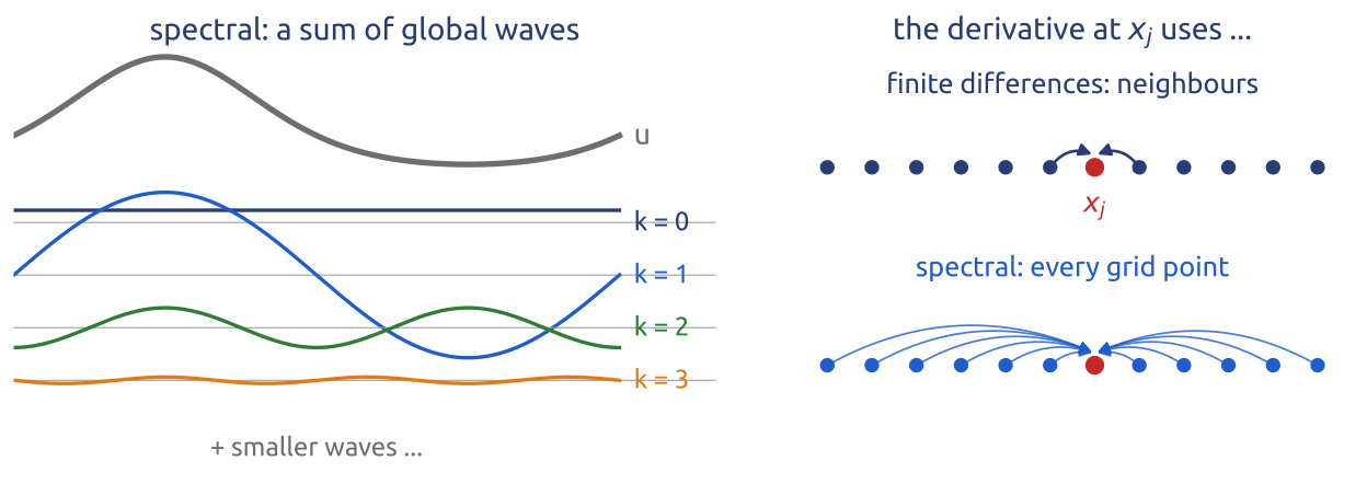
A finite-difference scheme approximates a derivative at a point from a few neighbours: it fits a local polynomial. A spectral method writes the whole field as a sum of global functions. On a periodic interval of length \(2\pi\), \[ u(x) = \sum_k \hat u_k\,e^{ikx}, \] and every wave \(e^{ikx}\) spans the whole domain (Figure 3). A change of \(u\) at one point changes every coefficient; the derivative at one point depends on the values at all points. This makes spectral methods very accurate for smooth fields, and also explains their cost and their trouble with discontinuities (Durran 2010, Sect. 6.2; Fornberg 1996).
4 Spectral derivative (1/3): interpolate
Throughout, \(M\) is the number of grid points and \(N\) the largest wavenumber kept (the truncation). On \(M\) equally spaced points \(x_j = j\Delta x\), \(\Delta x = 2\pi/M\), \(j = 0, \dots, M-1\), the \(M\) values \(u_j\) and \(M\) coefficients \(\hat u_k\) are related by the discrete Fourier transform \[
\hat u_k = \frac{1}{M}\sum_{j=0}^{M-1} u_j\,e^{-ikx_j}, \qquad
u_j = \sum_{k=-M/2+1}^{M/2}\hat u_k\,e^{ikx_j} \qquad (M \text{ even}).
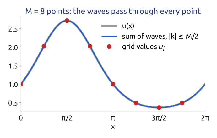
\] The second formula follows from the first by the discrete orthogonality \(\frac1M\sum_j e^{i(k-l)x_j} = 1\) if \(k - l\) is a multiple of \(M\), and 0 otherwise. Evaluated for any \(x\) (with the wave \(k = M/2\) taken as \(\hat u_{M/2}\cos(Mx/2)\), since on the grid it is \((-1)^j\)), the sum is a smooth periodic function that passes through every grid value: the trigonometric interpolant (Figure 4). The fast Fourier transform computes the \(M\) coefficients in \(O(M\log M)\) operations instead of \(M^2\) (Durran 2010, Sect. 6.2; Fornberg 1996). (numpy’s fft returns \(M\hat u_k\).)
5 Spectral derivative (2/3): differentiate
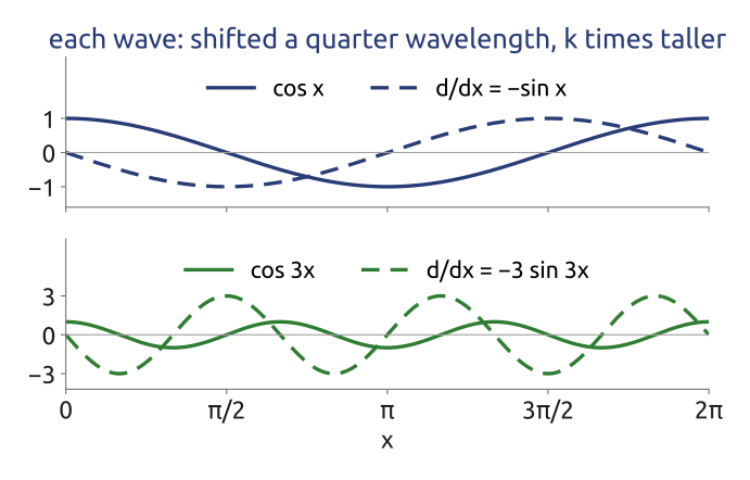
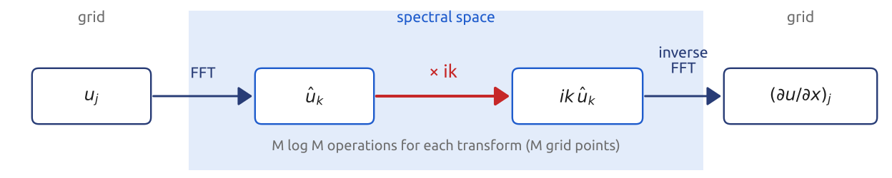
Differentiating the interpolant term by term, \[ \left(\frac{\partial u}{\partial x}\right)_j = \sum_k ik\,\hat u_k\,e^{ikx_j} , \] so the derivative is three steps: FFT, multiply each coefficient by \(ik\), inverse FFT (Figure 5). Each wave is shifted by a quarter wavelength and multiplied by \(k\). The wave \(k = M/2\) is \(\cos(Mx_j/2) = (-1)^j\) on the grid; the derivative of \(\cos(Mx/2)\) vanishes at the grid points, so its coefficient is set to zero (for the second derivative, \(-k^2\), it can be kept). In spectral space, \(\partial_x\) is a multiplication by \(ik\) and \(\nabla^2\) by \(-k^2\) (Durran 2010, Sect. 6.2).
6 Spectral derivative (3/3): all waves exact
Apply a derivative approximation to a single wave \(u = e^{ikx}\) in the advection equation \(u_t + c\,u_x = 0\). The centred second-order difference gives \[ \frac{e^{ik(x+\Delta x)} - e^{ik(x-\Delta x)}}{2\Delta x} = i\,\frac{\sin k\Delta x}{\Delta x}\,e^{ikx}, \qquad \omega = \frac{c\,\sin k\Delta x}{\Delta x}, \qquad \frac{c^*}{c} = \frac{\sin k\Delta x}{k\Delta x} \] (Durran 2010, Sect. 3.3.1), with the numerical phase speed \(c^* = \omega/k\); the fourth-order difference gives \(c^*/c = (8\sin k\Delta x - \sin 2k\Delta x)/(6k\Delta x)\). Both are close to 1 for long waves (\(k\Delta x \ll 1\)) and fall below it for short ones; the \(2\Delta x\) wave (\(k\Delta x = \pi\)) has \(c^* = 0\). The spectral derivative has \(c^* = c\) for every \(|k| < M/2\): it is exact for every wave the grid can carry (Figure 7, Figure 6).
7 How fast does the error fall?
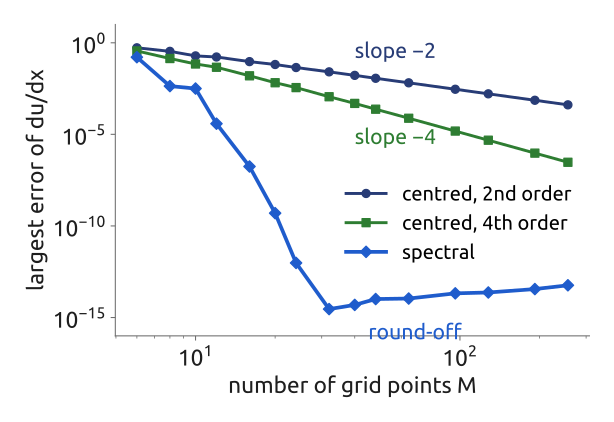
For the smooth function \(u = e^{\sin x}\), the largest error of \(\partial_x u\) with \(M = 32\) points is \(2.6\times10^{-2}\) for the centred second-order difference, \(1.1\times10^{-3}\) for the fourth-order one, and \(2.9\times10^{-15}\) (round-off) for the spectral derivative. The error of a scheme of order \(p\) falls like \(M^{-p}\); the spectral error falls faster than any power of \(M\) (Figure 8). A square wave, with jumps, rings (the Gibbs phenomenon) and converges slowly everywhere.
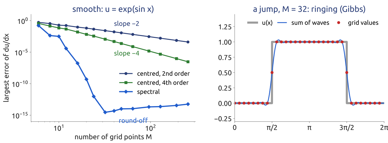
Mathematical aside: why. If \(u\) is periodic and \(p\) times continuously differentiable, integrating by parts \(p\) times gives \(|\hat u_k| \le C/|k|^p\). If \(u\) is analytic in a strip \(|\mathrm{Im}\,x| < \alpha\) of the complex plane, \(|\hat u_k| \le C e^{-\alpha|k|}\). The coefficients \(\tilde u_k\) computed from the grid values (the discrete Fourier transform) are the exact ones \(\hat u_k\) plus their aliases, \[ \tilde u_k = \sum_{r=-\infty}^{\infty}\hat u_{k+rM} \] (this follows from the discrete orthogonality), so the interpolant misses only the waves beyond \(M/2\) and their aliases, both of size about \(e^{-\alpha M/2}\), and the error of the derivative is of order \(M e^{-\alpha M/2}\): exponential convergence, “spectral accuracy” (Fornberg 1996; Durran 2010, Sect. 6.2.1). A function with a jump has \(|\hat u_k| \sim 1/|k|\): the interpolant oscillates near the jump and converges slowly, and because the waves are global the error is felt everywhere. Fronts, cloud edges, coastlines and steep orography are the hard cases for spectral models.
8 Advection without numerical dispersion
For the advection equation \(\partial_t u + c\,\partial_x u = 0\), the spectral method gives one ordinary differential equation per wave, \[ \frac{d\hat u_k}{dt} = -ick\,\hat u_k, \qquad \hat u_k(t) = \hat u_k(0)\,e^{-ickt} : \] every resolved wave moves at exactly \(c\), and there is no numerical dispersion in space; only the time stepping adds errors. With a centred difference the wave \(k\) moves at \(c^* = c\sin(k\Delta x)/(k\Delta x) < c\): the short waves that make up a narrow hump lag behind it and leave a trail of wiggles (Figure 9). Williamson (2007) notes this as one of the reasons spectral models dominated from the late 1970s: “linear advection is accurate to the truncation limit”. The weather, though, is nonlinear: \(\mathbf u\cdot\nabla\zeta\) is a product.
9 Derivatives, advection and aliasing, computed
A few lines of numpy (an FFT, a multiplication by \(ik\), an inverse FFT) are enough to measure these properties: how fast the coefficients of a smooth field, a field with a kink and one with a jump fall; the error of the spectral derivative against the centred differences of order 2 and 4, whose slopes \(-2\) and \(-4\) follow from their order; the advection of a hump for 1 and 10 revolutions, and the largest stable time step; and, once products are introduced, aliasing in \(u^2\) on a small grid and Burgers’ equation with and without the 2/3 rule (Figure 10).
10 A few waves do the work of many grid points
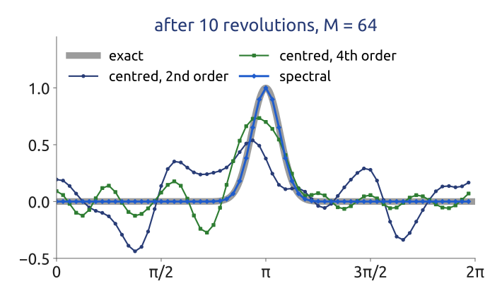
The errors of \(\partial_x u\) for \(u = e^{\sin x}\) with \(M = 32\) are \(2.6\times10^{-2}\) (centred, second order), \(1.1\times10^{-3}\) (fourth order) and \(2.9\times10^{-15}\) (spectral). After 10 revolutions of the hump the errors are 0.65, 0.36 and \(6\times10^{-5}\) (Figure 11). The price is a shorter time step. The fastest spectral wave has frequency \(|\omega| = c\,k_{\max} \approx c\pi/\Delta x\), against \(c/\Delta x\) for the centred difference. With RK4, stable for \(|\omega|\Delta t \le 2\sqrt2\), the spectral method needs a Courant number \(c\Delta t/\Delta x \lesssim 2\sqrt2/\pi \approx 0.9\), the centred difference \(\lesssim 2.8\): the shortest waves move at full speed. For smooth fields, a few waves do the work of many grid points. A kink (\(|\sin x|\)) makes the spectral error away from the kink only about \(1/M\): a defect spreads over the whole domain.
11 Products (1/3): two waves make new waves
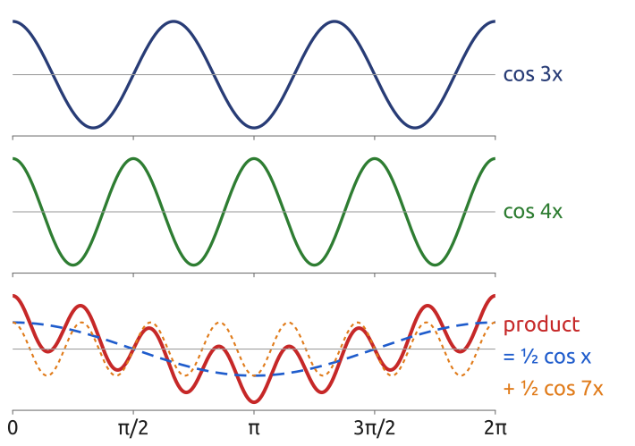
The equations are nonlinear: \(u\,\partial_x u\), \(\mathbf u\cdot\nabla\zeta\). A product of two waves is \(e^{ikx}e^{ilx} = e^{i(k+l)x}\); for example \(\cos 3x\cos 4x = \tfrac12\cos x + \tfrac12\cos 7x\): sum and difference waves (Figure 12). If \(u = \sum_l \hat u_l e^{ilx}\) and \(v = \sum_l \hat v_l e^{ilx}\) contain the waves \(|l| \le N\), every pair of waves \(l\) and \(k - l\) makes the wave \(k\): \[ u\,v = \sum_k \Big(\sum_l \hat u_l\,\hat v_{k-l}\Big)\,e^{ikx}, \qquad \widehat{(uv)}_k = \sum_l \hat u_l\,\hat v_{k-l} , \] so the product contains waves up to \(|k| = 2N\), and in spectral space it is a convolution, which costs \(O(N^2)\) operations per product in one dimension, and much more on the sphere, where the interaction coefficients of spherical harmonics must be stored. Silberman (1954) integrated the barotropic vorticity equation in spherical harmonics in this way, the first spectral model in meteorology (Ehrendorfer 2012, Sect. 7.3); Robert (1966) did the same for the primitive equations, at very low resolution. The cost kept spectral models small until 1970.
12 Products (2/3): the transform method
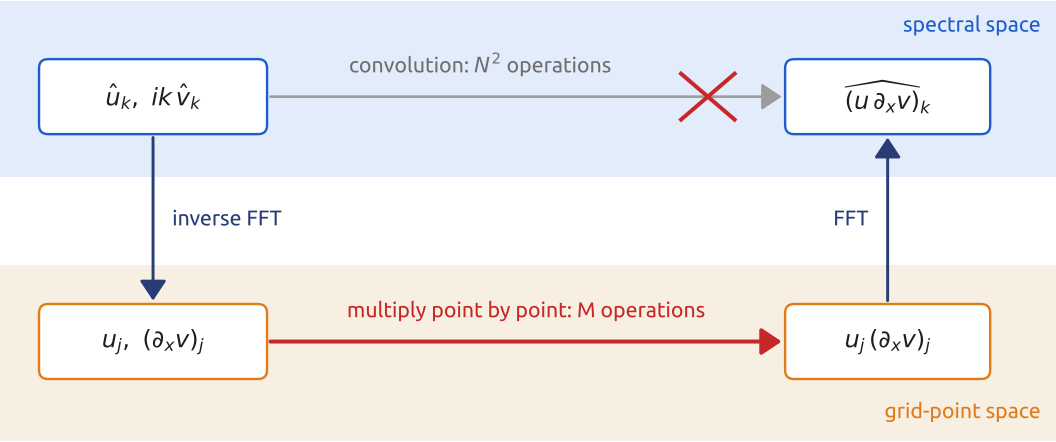
The transform method (Orszag 1970; Eliasen et al. 1970): compute the product on the grid. From the coefficients of \(u\) and of \(\partial_x v\), two inverse FFTs give their grid values; multiply them point by point (\(M\) operations); one FFT gives the coefficients of the product. The cost is \(O(M\log M)\). Derivatives and other linear operators are applied in spectral space, products on the grid: the pseudo-spectral or spectral transform method (Durran 2010, Sects. 6.2.2 and 6.3) (Figure 13). It made spectral models cost-effective, and from the mid to late 1970s it dominated global weather and climate modelling (Williamson 2007). (Names differ between books: Durran (2010) calls pseudospectral the collocation version, with as many grid points as waves, which aliases, and keeps spectral for the version with enough grid points to remove aliasing; Ehrendorfer (2012, Sect. 7.7) and the weather-prediction literature speak of the spectral transform method in both cases.) The product has waves up to \(2N\), with \(N\) the truncation, but a grid of \(M\) points carries only the waves \(|k| \le M/2\): where do the others go?
13 Products (3/3): aliasing
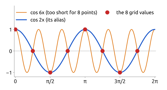
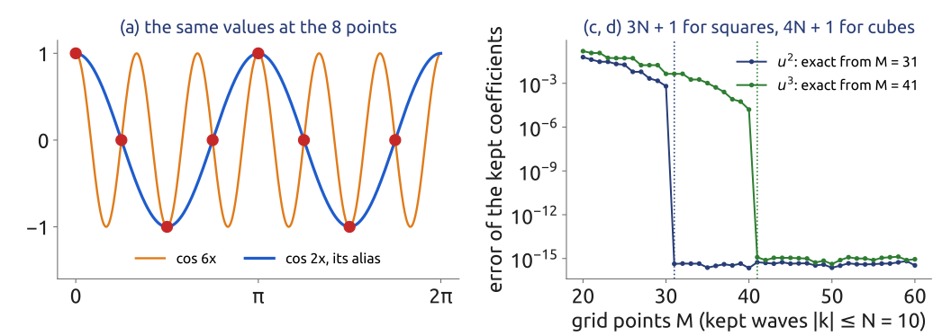
On a grid of \(M\) points, \(e^{i(k+M)x_j} = e^{ikx_j}e^{iMx_j} = e^{ikx_j}\), because \(Mx_j = 2\pi j\). The waves \(k\) and \(k \pm M\) take the same values at every grid point: the grid cannot tell them apart, and a wave too short for the grid is seen as a longer one, its alias (Figure 14). On 8 points, for example, \(\cos 6x_j = \cos(6-8)x_j = \cos 2x_j\). In terms of coefficients: if \(u(x) = \sum_k \hat u_k e^{ikx}\) exactly, the coefficients computed from the \(M\) grid values are \[ \tilde u_k = \frac{1}{M}\sum_{j=0}^{M-1} u_j\,e^{-ikx_j} = \sum_{r=-\infty}^{\infty}\hat u_{k+rM} , \] by the discrete orthogonality: each computed coefficient is the exact one plus the exact coefficients of all its aliases. For \(u = \cos 6x\) (\(\hat u_{\pm6} = \tfrac12\)) on 8 points, \(\tilde u_{\pm 2} = \tfrac12\) and \(\tilde u_{\pm 6}\) does not exist: the grid sees \(\cos 2x\). When a product is computed on the grid, its waves beyond the grid’s range come back as aliases on the kept waves: wrong energy at small scales. In a nonlinear model this can grow without bound: the nonlinear instability found by Phillips in 1959 in a finite-difference model (Durran 2010, Sect. 4.5, 6.3; Ehrendorfer 2012, Sect. 7.9–7.10).
14 The 2/3 rule
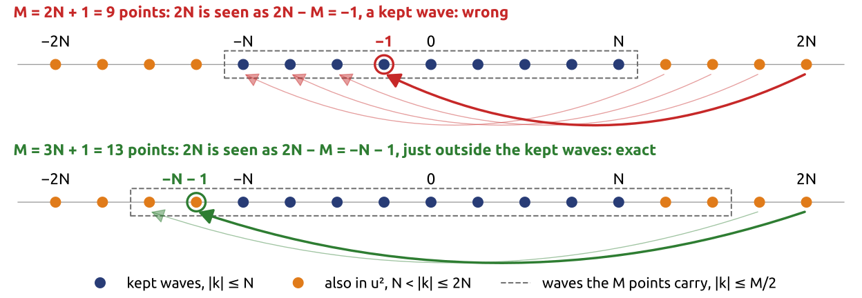
Suppose \(u\) and \(v\) keep the waves \(|k| \le N\) and the product is computed on \(M\) points. The product has waves up to \(2N\); the wave \(2N\) is seen as \(2N - M\). To keep every alias away from the kept waves we need \(2N - M < -N\), that is \[ M \ge 3N + 1 . \] The waves of the product between \(N\) and \(M/2\) are represented on the grid and simply dropped by the truncation; those beyond \(M/2\) alias onto \(k \le -N - 1\) and are dropped too. So with three grid points per shortest kept wave the kept coefficients of a quadratic product are exact. Equivalently, on a given grid of \(M\) points one keeps only the waves \(|k| < M/3\), the lower two thirds: the “2/3 rule” (Orszag 1971; Durran 2010, Sect. 6.3). For T42 this gives \(3\cdot42 + 1 = 127\), and the T42 grid has 128 longitudes (Figure 15). The IFS names its grids by the number of points per shortest wave: linear (2), quadratic (3), cubic (4).
15 In class: aliasing on a small grid
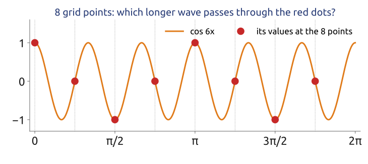
Exercise 1 — Aliasing on a small grid. Take the \(M = 8\) grid points \(x_j = 2\pi j/8\). (a) Show that \(\cos 6x_j = \cos 2x_j\) at every grid point. Which waves look like \(k = 1\) on this grid? (b) \(u = \cos 3x\) is carried by the grid. What does the grid see for \(u^2 = \tfrac12 + \tfrac12\cos 6x\)? (c) A field keeps the waves \(|k| \le N\). How many points \(M\) are needed so that no alias of \(u^2\) falls on a kept wave? Check T42 and its 128 longitudes.
(d) To hand in: cubic products. The same question for \(u^3\). Which fraction of the grid’s waves can be kept? ECMWF’s model uses a “cubic” grid, with four points per shortest wave: why the name?
16 What the exercise showed
- On 8 points \(k\) and \(k \pm 8\) agree: \(\cos 6x_j = \cos(-2x_j) = \cos 2x_j\), and \(k = 1\) looks like \(9, -7, 17, \dots\) (b) \(u^2 = \tfrac12 + \tfrac12\cos 6x\) is seen as \(\tfrac12 + \tfrac12\cos 2x\): a wave that is not in \(u^2\) at all. (c) The alias of \(2N\) is \(2N - M\), which must be below \(-N\): \(M \ge 3N + 1\); T42: \(127 \le 128\) longitudes. (d) \(u^3\) has waves up to \(3N\), so \(M \ge 4N + 1\): keep half of the grid’s waves; the “cubic” grid of the ECMWF model, with four points per shortest wave, computes cubic products without aliasing on the kept waves. A check with a random field of waves \(|k| \le 10\) (Figure 17): the error of the kept coefficients drops to round-off at \(M = 31\) for \(u^2\) and \(M = 41\) for \(u^3\).
17 From the plane to the sphere
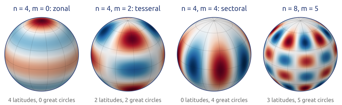
On the sphere a Fourier series in longitude is natural (it is periodic), but not in latitude: the sphere is not periodic in latitude, and a latitude–longitude grid crowds its points near the poles. The natural functions are the spherical harmonics \[ Y_n^m(\lambda, \mu) = P_n^m(\mu)\,e^{im\lambda}, \qquad \mu = \sin\varphi, \qquad 0 \le |m| \le n , \] a Fourier wave in longitude \(\lambda\) (zonal wavenumber \(m\)) times an associated Legendre function of latitude \(\varphi\) (\(n\) is the total wavenumber). We normalize so that \(\tfrac12\int_{-1}^1 (P_n^m)^2\,d\mu = 1\); then the \(Y_n^m\) are orthonormal for the average over the sphere. The sign convention is the one of the ECMWF model: \(P_n^m \ge 0\) near the north pole for \(m \ge 0\), without the factor \((-1)^m\) (Condon–Shortley phase) of many textbooks, and \(P_n^{-m} = P_n^m\) (Ehrendorfer 2012, App. B.1 and B.3 (footnote 164: the sign is chosen “to conform with the sign convention used at ECMWF”); ECMWF 2026, Sect. 2.2.4). Durran writes \(Y_{m,n}\), with the order first, for the same functions with another normalisation (Durran 2010, Sect. 6.4). The real part of \(Y_n^m\) has \(n - |m|\) nodal circles of latitude and \(|m|\) nodal great circles through the poles: \(n\) nodal lines in all (Figure 18). Harmonics with \(m = 0\) are called zonal, with \(|m| = n\) sectoral, the others tesseral. They are smooth everywhere, poles included.
18 On the sphere (1/3): the Poisson problem
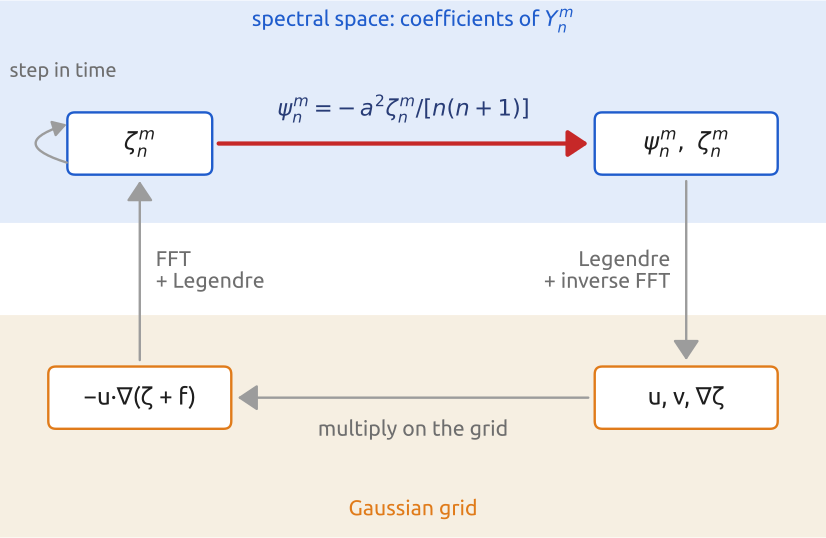
The barotropic vorticity equation on the rotating sphere is \[ \frac{\partial\zeta}{\partial t} + \mathbf u\cdot\nabla(\zeta + f) = 0, \qquad \zeta = \nabla^2\psi, \qquad u = -\frac{1}{a}\frac{\partial\psi}{\partial\varphi}, \quad v = \frac{1}{a\cos\varphi}\frac{\partial\psi}{\partial\lambda}, \] with \(f = 2\Omega\sin\varphi = 2\Omega\mu\) and \(a\) the radius of the Earth; in the plane, \(\mathbf u\cdot\nabla q = J(\psi, q) = \psi_x q_y - \psi_y q_x\), and on the sphere \(\mathbf u\cdot\nabla q = [\psi_\lambda q_\varphi - \psi_\varphi q_\lambda]/(a^2\cos\varphi)\). The Laplacian in \(\zeta = \nabla^2\psi\) is the spherical Laplacian; in longitude \(\lambda\) and latitude \(\varphi\) (Vallis 2017), \[ \nabla^2 f = \frac{1}{a^2\cos\varphi}\frac{\partial}{\partial\varphi}\Big(\cos\varphi\,\frac{\partial f}{\partial\varphi}\Big) + \frac{1}{a^2\cos^2\varphi}\frac{\partial^2 f}{\partial\lambda^2} . \] Spherical harmonics are its eigenfunctions: in the coordinates \((\lambda, \mu)\), with \(\mu = \sin\varphi\), \[ \nabla^2 f = \frac{1}{a^2}\left[\frac{\partial}{\partial\mu}\Big((1-\mu^2)\frac{\partial f}{\partial\mu}\Big) + \frac{1}{1-\mu^2}\frac{\partial^2 f}{\partial\lambda^2}\right], \] and \(P_n^m\) solves the associated Legendre equation \(\frac{d}{d\mu}\big[(1-\mu^2)\frac{dP}{d\mu}\big] - \frac{m^2}{1-\mu^2}P = -n(n+1)P\), so that \[ \nabla^2 Y_n^m = -\frac{n(n+1)}{a^2}\,Y_n^m, \qquad \psi_n^m = -\frac{a^2}{n(n+1)}\,\zeta_n^m \qquad (n \ge 1), \] with \(\psi_0^0\) arbitrary (set to zero). The eigenvalue depends on \(n\) only: \(n\) sets the scale (a wavelength of about \(2\pi a/n\): about 950 km for T42, 31 km for T1279), \(m\) only the orientation. The 1950 Poisson problem is a division, as with von Neumann’s sines (Ehrendorfer 2012, Sect. 7.14; ECMWF 2026, Sect. 2.2.4). Expand \(\zeta = \sum_{n=0}^N\sum_{m=-n}^n \zeta_n^m Y_n^m\); with the sign convention above, for a real field, \(\zeta_n^{-m} = (\zeta_n^m)^*\) (with the Condon–Shortley phase it would be \((-1)^m(\zeta_n^m)^*\) (Ehrendorfer 2012, eq. 7.157; Durran 2010, eq. 6.49)), and only \(m \ge 0\) is stored (Figure 19).
19 On the sphere (2/3): to the grid and back
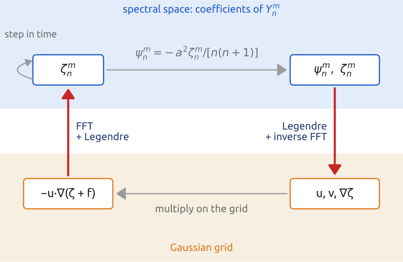
The velocity looks singular at the poles in \((u, v)\), but \(U = u\cos\varphi\) and \(V = v\cos\varphi\) are smooth: \[ U = -\frac{1}{a}(1-\mu^2)\frac{\partial\psi}{\partial\mu}, \qquad V = \frac{1}{a}\frac{\partial\psi}{\partial\lambda} . \] The \(\lambda\) derivative multiplies each coefficient by \(im\). The \(\mu\) derivative uses the recursion \[ (1-\mu^2)\frac{dP_n^m}{d\mu} = -n\,\varepsilon_{n+1}^m P_{n+1}^m + (n+1)\,\varepsilon_n^m P_{n-1}^m, \qquad \varepsilon_n^m = \sqrt{\frac{n^2 - m^2}{4n^2 - 1}} , \] so \(U\), \(V\), \(\partial\zeta/\partial\lambda\) and \(\cos\varphi\,\partial\zeta/\partial\varphi\) are computed exactly on the grid by inverse transforms: for each \(m\), a sum over \(n\) (the inverse Legendre transform) at each latitude, then an inverse FFT along each latitude circle. The direct transform goes back: an FFT along each latitude circle gives \(X_m(\mu) = \frac{1}{2\pi}\int_0^{2\pi}X\,e^{-im\lambda}d\lambda\), then a Legendre transform \(X_n^m = \tfrac12\int_{-1}^1 X_m(\mu)P_n^m(\mu)\,d\mu\), computed by Gaussian quadrature, \[ X_n^m = \sum_{j=1}^{N_{lat}} w_j\,X_m(\mu_j)\,P_n^m(\mu_j), \] with the Gaussian latitudes \(\mu_j\), the roots of the Legendre polynomial \(P_{N_{lat}}\), and their weights \(w_j\), normalised to sum to 1 as in the IFS documentation. The quadrature is exact for polynomials in \(\mu\) of degree up to \(2N_{lat} - 1\) (ECMWF 2026, Sect. 2.2.4; Ehrendorfer 2012, Sect. 7.11). For the product of two fields of truncation \(N\), the integrand is a polynomial of degree up to about \(3N\), which gives the quadratic Gaussian grid: \(N_{lat} \ge (3N+1)/2\) latitudes and \(3N + 1\) longitudes, the spherical form of the 2/3 rule (Figure 20).
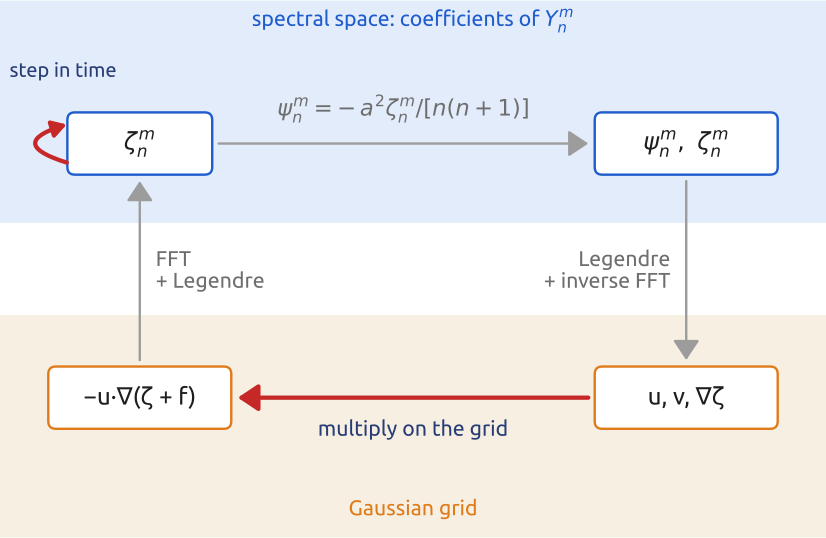
20 On the sphere (3/3): one time step
On the grid, \[ \mathbf u\cdot\nabla(\zeta + f) = \frac{1}{a\cos^2\varphi}\left[U\frac{\partial\zeta}{\partial\lambda} + V\Big(\cos\varphi\frac{\partial\zeta}{\partial\varphi} + 2\Omega\cos^2\varphi\Big)\right], \] then a direct transform gives its coefficients, and each coefficient is stepped in time: \[ \frac{d\zeta_n^m}{dt} = -\big[\mathbf u\cdot\nabla(\zeta + f)\big]_n^m - \nu_4\Big(\frac{n(n+1)}{a^2}\Big)^2\zeta_n^m , \] where \([\,\cdot\,]_n^m\) is the coefficient of \(Y_n^m\) and the last term, a \(\nabla^4\) hyperdiffusion with coefficient \(\nu_4\), removes the enstrophy that cascades to the smallest scales (Ehrendorfer 2012, Sect. 7.14). Linear operators are numbers in spectral space, products are computed on the grid: the barotropic vorticity equation on the whole sphere (Figure 21). The time stepping can be leapfrog or a Runge–Kutta scheme.
21 Triangular truncation and the Gaussian grid
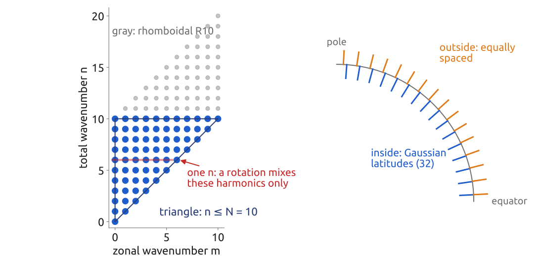
Keeping all \(Y_n^m\) with \(0 \le |m| \le n \le N\) is the triangular truncation \(N\) (the model is called T\(N\)). It is isotropic: the resolution is the same in every direction and at every place on the sphere. The reason is that the Laplacian commutes with rotations of the sphere, so each eigenspace (all the \(Y_n^m\) of one \(n\), \(2n+1\) functions) is mapped into itself by a rotation: rotating the sphere mixes the \(m\) of one \(n\), never different \(n\). A truncation that cuts at a fixed \(n\) is therefore unchanged by a rotation; a rhomboidal truncation (\(|m| \le N\), \(n - |m| \le N\), used in early models) is not (Ehrendorfer 2012, Sect. 7.11; Durran 2010, Sect. 6.4.1). The quadratic grid for T42 has 64 latitudes and 128 longitudes. The shortest wave of truncation T\(N\) has a wavelength of about \(2\pi a/N\): about 950 km for T42. The grid spacing is smaller (two to four points per shortest wave), which is why the resolution of a spectral model is quoted in two ways (Figure 22). Gaussian latitudes are almost equally spaced, a little closer near the poles.
22 In class: Rossby–Haurwitz waves
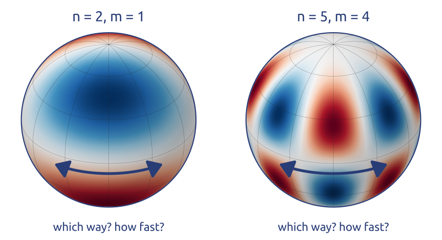
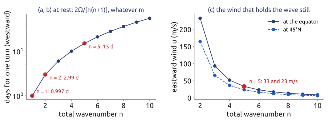
Exercise 2 — Rossby–Haurwitz waves. On the sphere, the barotropic vorticity equation linearized about rest is \(\partial_t\nabla^2\psi + (2\Omega/a^2)\,\partial_\lambda\psi = 0\). Take \(\psi = A\,P_n^m(\sin\varphi)\cos(m\lambda - \sigma t)\). (a) With \(\nabla^2 Y_n^m = -n(n+1)Y_n^m/a^2\), find \(\sigma\) and the angular speed \(\sigma/m\) of the pattern. East or west? (b) How many days does it take to go once round the Earth for \(n = 1, 2, 5\)? What is special about \(n = 1\)?
(c) To hand in: a stationary wave. Add an eastward wind in solid-body rotation, \(u = \omega a\cos\varphi\) (the air turns a little faster than the Earth). The pattern then turns at \(\omega - 2(\Omega + \omega)/[n(n+1)]\). Which \(\omega\) makes the wave \(n = 5\) stationary? What is \(u\) at the equator and at \(45^\circ\)N?
23 What the exercise showed
- With \(\psi = A P_n^m\cos(m\lambda - \sigma t)\), \(\partial_t\nabla^2\psi = -\frac{n(n+1)}{a^2}\,\sigma A P_n^m\sin(m\lambda - \sigma t)\) and \(\frac{2\Omega}{a^2}\partial_\lambda\psi = -\frac{2\Omega}{a^2}\,m A P_n^m\sin(m\lambda - \sigma t)\). Their sum vanishes if \(\sigma = -2\Omega m/[n(n+1)]\): the pattern turns at the angular speed \(\sigma/m = -2\Omega/[n(n+1)]\), westward, and the speed depends on \(n\) only (Haurwitz 1940): the largest scales are the fastest. (b) Once round the Earth in \(\pi n(n+1)/\Omega\): 0.997 days for \(n = 1\), 3.0 days for \(n = 2\), 15 days for \(n = 5\). For \(n = 1\) the pattern turns westward once a day relative to the Earth, so it is fixed in space: a harmonic with \(n = 1\), \(m = 1\) is a solid-body rotation about a tilted axis, which the Earth turns under. (c) The pattern is stationary when \(\omega - 2(\Omega + \omega)/[n(n+1)] = 0\), \(\omega = 2\Omega/[n(n+1) - 2]\); for \(n = 5\), \(\omega = \Omega/14 = 5.2\times10^{-6}\) s\(^{-1}\), so \(u = \omega a\cos\varphi = 33\) m/s at the equator and 23 m/s at \(45^\circ\)N: Rossby’s stationary waves (Figure 24). These Rossby–Haurwitz waves are the spherical version of the Rossby waves of the \(\beta\)-plane. (In the test case of Williamson et al. (1992) the wave is written with \(R\), \(\omega\), \(K\) and an angular speed \(\nu\): their zonal wavenumber \(R\) is our \(m\), the harmonic has \(n = R+1\), and \(\nu\) is not the hyperdiffusion coefficient \(\nu_4\).)
24 The barotropic vorticity equation, computed on a plane and on the sphere
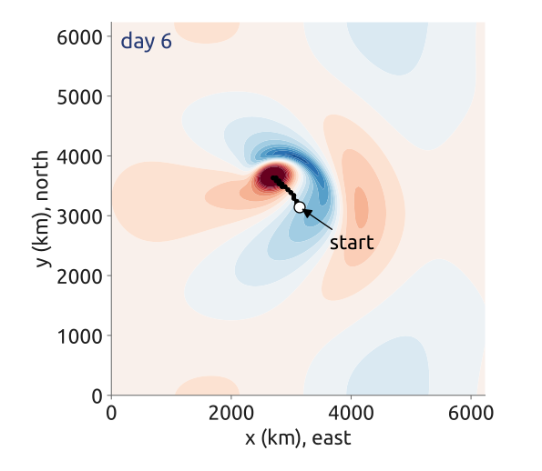
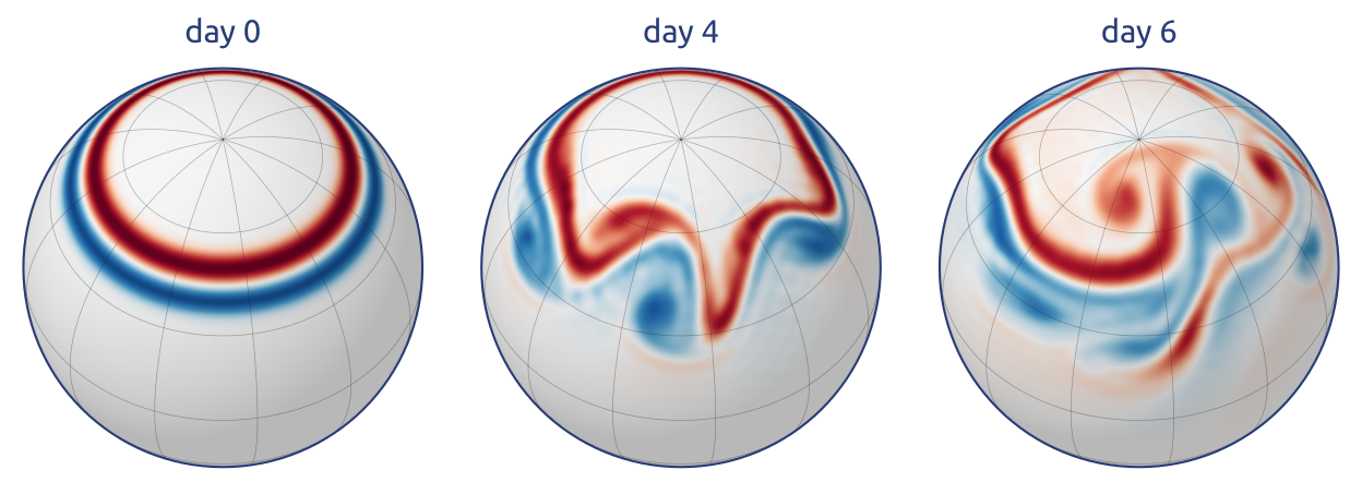
The same pseudo-spectral model of the barotropic vorticity equation runs on a doubly periodic \(\beta\)-plane and, with spherical harmonics, on the sphere. On the plane it reproduces the Rossby-wave frequencies \(\omega = -\beta k/(k^2 + l^2)\), follows a single cyclone, and, over longer runs, two-dimensional turbulence. On the sphere it builds the transform in a few lines (Gaussian latitudes, Legendre functions by recursion, FFTs), checks the Rossby–Haurwitz waves, and runs an unstable jet (Figure 25).
25 Model against exact solutions: Rossby waves, a drifting cyclone, an unstable jet
On the plane, the model’s Rossby-wave frequencies equal \(-\beta k/(k^2 + l^2)\) to all printed digits. The cyclone drifts north-west at about 1 m/s (the \(\beta\) drift), leaving Rossby waves behind. The Rossby–Haurwitz wave of Williamson’s test case moves 122° east in 10 days with an error of \(10^{-8}\) (only the time stepping), and at rest the waves move westward at \(2\Omega/[n(n+1)]\). The unstable jet, of the shape of Galewsky et al. (2004), grows from a tiny bump into breaking waves in 4–6 days; T42 and T63 disagree by day 6 (Figure 26). On a laptop a forecast day takes seconds; on the ENIAC it took a day. A spectral model of the barotropic vorticity equation on the whole sphere fits in about sixty lines of numpy.
26 Semi-implicit (1/2): the gravity-wave limit
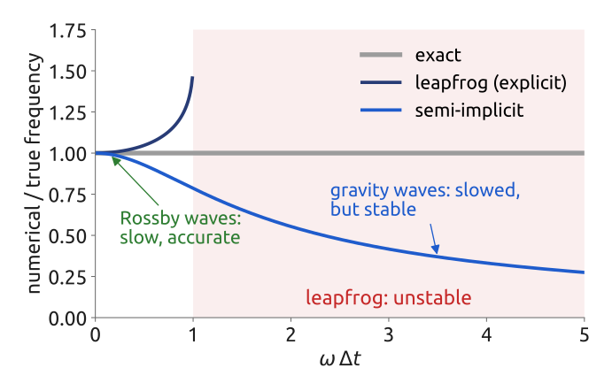
The barotropic vorticity equation has no gravity waves. The shallow water and primitive equations do: external gravity waves move at \(\sqrt{gH} \approx 300\) m/s, ten times faster than the wind, and with an explicit scheme they set the time step through the CFL condition, although they carry little energy. Take the linear shallow water equations without rotation, \(\partial_t\mathbf u = -g\nabla \eta\), \(\partial_t \eta = -H\nabla\cdot\mathbf u\), with \(\eta\) the height perturbation and \(H\) the mean depth. The divergence of the first, with \(\delta = \nabla\cdot\mathbf u\), gives the pair \[ \frac{\partial\delta}{\partial t} = -g\nabla^2 \eta, \qquad \frac{\partial \eta}{\partial t} = -H\delta , \] and eliminating \(\eta\), \(\partial_{tt}\delta = gH\nabla^2\delta\): gravity waves at the speed \(\sqrt{gH}\). Robert’s semi-implicit scheme treats the linear terms that make gravity waves implicitly, as averages of the values at \(t - \Delta t\) and \(t + \Delta t\), and the rest explicitly (Staniforth 1997; Durran 2010, Sect. 8.2). For an oscillation \(dF/dt = i\omega F\), leapfrog is stable only for \(\omega\Delta t \le 1\), with \(\sin(\omega_{\text{num}}\Delta t) = \omega\Delta t\), while the averaged treatment gives \(\tan(\omega_{\text{num}}\Delta t) = \omega\Delta t\), stable for every \(\Delta t\): slow waves are accurate, fast gravity waves are slowed down but harmless (Figure 27). Robert’s idea started, Staniforth tells, at a seminar on implicit methods by G. I. Marchuk.
27 Semi-implicit (2/2): Helmholtz, a division
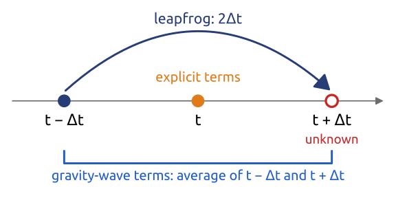
With the other terms (nonlinear, Coriolis) collected in \(R_\delta\) and \(R_h\) and treated explicitly, the leapfrog step with the linear terms averaged is (with \(\pm\) for the time levels \(t \pm \Delta t\), to keep \(n\) for the total wavenumber) \[ \delta^{+} = \delta^{-} - g\Delta t\,\nabla^2\big(\eta^{+} + \eta^{-}\big) + 2\Delta t R_\delta, \qquad \eta^{+} = \eta^{-} - H\Delta t\,\big(\delta^{+} + \delta^{-}\big) + 2\Delta t R_h . \] Eliminating \(\eta^{+}\) gives a Helmholtz equation for \(\delta^{+}\), \[ \big(1 - gH\Delta t^2\,\nabla^2\big)\,\delta^{+} = R , \] with \(R\) everything known at \(t\) and \(t - \Delta t\); in spherical harmonics it is again a division: \(\delta_n^{m,+} = R_n^m / \big[1 + gH\Delta t^2\,n(n+1)/a^2\big]\). “This is negligible for a spectral model”, as Staniforth writes of the cost of the Helmholtz problem (Staniforth 1997, 35). A grid-point model must instead solve an elliptic problem on the whole globe at every step, usually by an iterative method. In a model with many levels, the gravity-wave terms couple the levels through the hydrostatic relation, and the Helmholtz problem becomes, for each \((m, n)\), a small linear system \(\big[I + \tfrac{n(n+1)}{a^2}\Gamma\big]D_n^{m,+} = \tilde D_n^m\) for the divergence at all levels at \(t + \Delta t\), where \(\Gamma\) is a matrix of the size of the number of levels (ECMWF 2026, Sect. 2.2.7, Eq. 2.50; Durran 2010, Sect. 8.2.3). Its eigenvectors are vertical normal modes, and its eigenvalues, \(gh_k\Delta t^2\) up to a constant factor, give their equivalent depths \(h_k\): in the basis of the modes the system splits into one Helmholtz problem, and one division, per mode.
28 The grids of the IFS
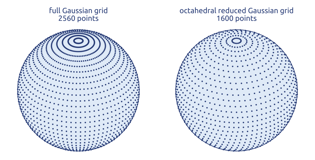
Near the poles a harmonic of large \(m\) is tiny, so fewer points per latitude circle are needed there: the Gaussian grid of the ECMWF model is reduced towards the poles since 1991 (Hortal and Simmons 1991). Since March 2016 the grid is octahedral: 20 points on the latitude next to each pole and 4 more on each latitude towards the equator (ECMWF 2026, Sect. 2.2.5; Malardel et al. 2016). For 1280 latitudes per hemisphere this gives \(2\sum_{i=1}^{1280}(20 + 4(i-1)) = 6\,599\,680\) points per level, against about 8.5 million for the earlier reduced grid: 22% cheaper. The grid paired with truncation \(N\) has 2, 3 or 4 points per shortest wave (linear, quadratic, cubic). The quadratic grid (the 2/3 rule) was used until 1998; the semi-Lagrangian scheme allowed the cheaper linear grid; at high resolution aliasing came back, and in 2016 ECMWF moved to the cubic grid, which has almost no aliasing: TCo1279 is truncation 1279 on the cubic octahedral grid with 1280 latitudes per hemisphere, about 9 km (ECMWF 2026, Sect. 2.2.6; Malardel et al. 2016) (Figure 29). A spectral model can drop points near the poles because the truncation already removes the short waves there; a latitude–longitude finite-difference model cannot.
29 IFS today
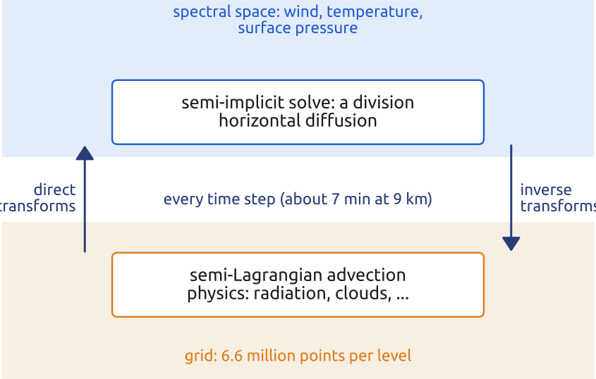
The Integrated Forecasting System of ECMWF has been a spectral model since April 1983, when ECMWF’s first spectral model went into operations (ECMWF 2026, Sect. 2.2.4). Its current cycle (Cy50r1, operational since 12 May 2026) runs the medium-range forecasts at TCo1279, a grid spacing of about 9 km, with 137 levels up to 0.01 hPa, and an ensemble of 50 members plus a control at the same resolution (ECMWF model information page, Cy50r1). The main ingredients (Figure 30):
- Spectral transform. The wind, the virtual temperature and the surface pressure go to spectral space and back at every time step; specific humidity, clouds and tracers stay on the grid, since transforms can create negative values in non-smooth fields (ECMWF 2026, Sect. 2.2.4).
- Semi-Lagrangian advection. Instead of the Eulerian \(\mathbf u\cdot\nabla\), each grid point looks back along the trajectory to its departure point and interpolates the field there. This is stable for long time steps.
- Semi-implicit time stepping, with the Helmholtz problem solved in spectral space. Together, a time step of several minutes at 9 km: 400 s in Malardel et al. (2016).
30 The cost of the transforms
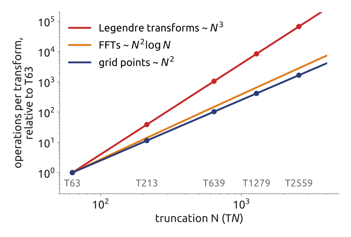
For triangular truncation \(N\) on a quadratic grid there are about \(N^2/2\) coefficients \((m, n)\) with \(m \ge 0\) and about \(1.5\,N\) latitudes, so a Legendre transform of one field costs about \(0.75\,N^3\) operations, while the FFTs cost \(O(N^2\log N)\) and the grid has \(O(N^2)\) points (Williamson 2007) (Figure 31). Doubling the resolution multiplies the grid by 4, the Legendre work by 8, and halves the time step. Fast Legendre transforms that exploit the structure of the \(P_n^m\) reduce this cost substantially at high resolution (Wedi et al. 2013). The harder problem is communication: every coefficient depends on every grid point, so each transform requires a global exchange of data (“transpositions”) across the whole supercomputer, at every time step. In the words of the IFS documentation, these “remain a concern on future computing architectures” (ECMWF 2026, Sect. 2.2.4). Methods that only exchange data with neighbours, finite volumes and finite elements on quasi-uniform grids, are the alternative.
31 Spectral models today
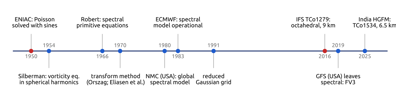
Spectral models are not a thing of the past (Figure 32). Besides the IFS, Météo-France’s global model ARPEGE is spectral on a stretched sphere: a conformal (Schmidt) transformation moves the pole of the harmonics over France and concentrates the resolution there (Courtier and Geleyn 1988); in 2016 it ran at T1198 with a stretching factor 2.2, from about 7 km over France to 33 km over the South Pacific. Its limited-area relatives ALADIN and AROME are spectral on a plane: a Fourier series in \(x\) and \(y\) (bi-Fourier), made periodic by an extension zone added to the domain; AROME-France runs at 1.3 km (Météo-France 2016; Seity et al. 2011). The Global Spectral Model of the Japan Meteorological Agency (GSM) moved in March 2023 from a linear to a quadratic grid, TQ959, about 13 km, to reduce the small-scale noise of spectral blocking (Yonehara et al. 2025). In climate, the European Earth system model EC-Earth3 couples the IFS (the atmosphere and land, at T255 with 91 levels, about 80 km) to the ocean model NEMO and its sea ice; it is built by a consortium of 27 partners in ten European countries, in Italy the Institute of Atmospheric Sciences and Climate of the National Research Council (ISAC-CNR, Bologna and Turin), the energy agency ENEA (Rome) and the Politecnico di Torino (Döscher et al. 2022). The Brazilian Global Atmospheric Model of CPTEC (BAM) is a spectral, semi-implicit model (Eulerian or semi-Lagrangian), run at TQ0666, about 20 km (Figueroa et al. 2016); the High-Resolution Global Forecast Model of IITM, India (HGFM, the basis of the Bharat Forecast System), uses the cubic octahedral grid at TCo1534, about 6.5 km in the tropics (Krishna et al. 2025); China’s YHGSM (National University of Defense Technology) is a spectral model with semi-Lagrangian advection (Jiang et al. 2021). The United States went spectral first: the global spectral model of the National Meteorological Center (now NCEP) became operational in August 1980 (Sela 1980), three years before ECMWF’s; run as the AVN and MRF forecasts, it was renamed the Global Forecast System (GFS) in 2002, and it stayed spectral until June 2019, when it moved to the finite-volume cubed-sphere core FV3 (NCEP, GFS documentation). ECMWF also develops a finite-volume core (FVM) for the future.
32 A Galerkin method
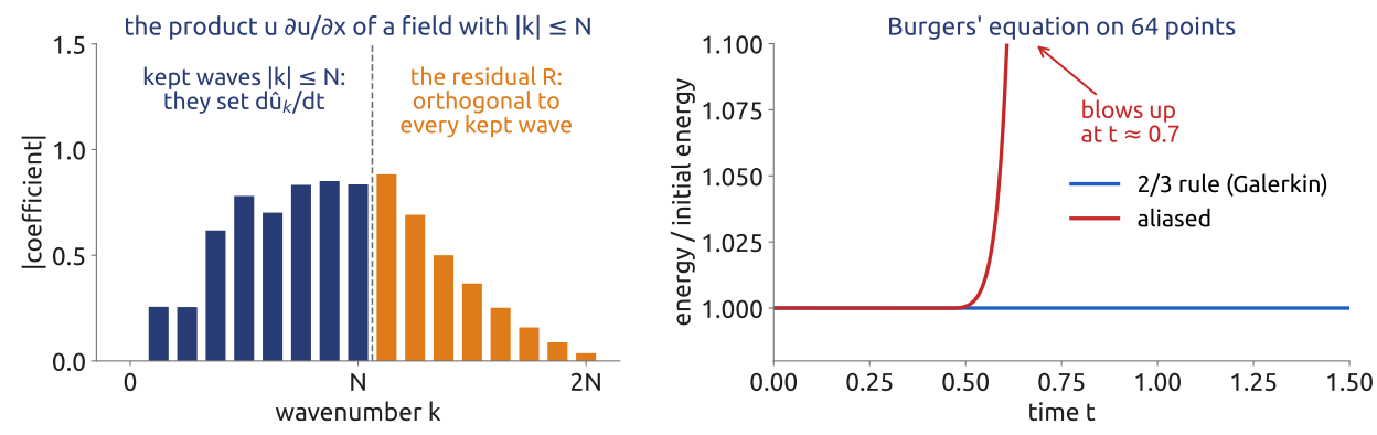
Following Durran (2010, Sect. 6.1), write the equation as \(\partial_t u + F(u) = 0\), with \(F\) the terms with space derivatives, and truncate the field to the kept waves, \(u_N = \sum_{|k| \le N}\hat u_k\,e^{ikx}\). The truncated field cannot satisfy the equation exactly: the product in \(F\) makes waves up to \(2N\) (Figure 33, left). What is left is the residual \(R = \partial_t u_N + F(u_N)\). The Galerkin approximation asks the residual to be orthogonal to every expansion function kept, \[ \int_0^{2\pi} R\,e^{-ikx}\,dx = 0 \qquad \text{for every } |k| \le N , \] which gives one ordinary differential equation per kept coefficient: \(d\hat u_k/dt\) is minus the coefficient \(k\) of \(F(u_N)\). This is the spectral method, and the transform method computes it exactly when the products are not aliased (the 2/3 rule): the waves of the product beyond \(N\), the residual, are dropped.
The Galerkin condition conserves what the equation conserves (Durran 2010, Sect. 6.2.3). Let \(P_N\) be the orthogonal projection onto the waves \(|k| \le N\). For Burgers’ equation the dealiased spectral method is \(\partial_t u_N = -P_N(u_N\,\partial_x u_N)\), and \[ \frac{d}{dt}\,\frac12\int u_N^2\,dx = -\int u_N\,P_N(u_N\,\partial_x u_N)\,dx = -\int u_N^2\,\partial_x u_N\,dx = -\int \partial_x\Big(\frac{u_N^3}{3}\Big)dx = 0 , \] because \(P_N\) is self-adjoint and \(P_N u_N = u_N\). The energy is conserved whatever the nonlinearity, so there is no nonlinear instability; only the time stepping can add errors. With aliasing the computed product is not \(P_N(u_N\,\partial_x u_N)\) and the identity fails: on 64 points the aliased run blows up, the dealiased one keeps its energy (Figure 33, right).
Finite elements use the same Galerkin condition with other expansion functions: instead of global waves, local functions, each non-zero on a few cells of a mesh of any shape (Durran 2010, Sect. 6.5).
33 Key points
- Spectral derivative: exact for every resolved wave; spectral accuracy for smooth fields; ringing at jumps.
- Transform method: products on the grid; aliasing; the 2/3 rule (\(3N + 1\) points).
- Spherical harmonics \(Y_n^m\): \(\nabla^2 Y_n^m = -n(n+1)Y_n^m/a^2\); triangular truncation \(N\) (T\(N\)); Gaussian grid; no pole problem.
- Poisson and Helmholtz problems are divisions: semi-implicit steps are cheap.
- Legendre transforms cost \(\sim N^3\) and need global communication: the scaling limit.
- The IFS: spectral, semi-Lagrangian, semi-implicit, 9 km.
- A Galerkin method: the residual is orthogonal to every kept wave; energy conserved without aliasing.
Spectral methods: exact derivatives and cheap implicit steps, at the price of global transforms. Still open: jumps and positive fields such as moisture, which the IFS keeps on the grid; and the global communication, which the Galerkin idea with local basis functions on any mesh, the finite elements, avoids.
Further reading
Durran (2010), Chapter 6 (spectral, pseudospectral, spherical harmonics) and Section 8.2 (semi-implicit); Ehrendorfer (2012), a whole book on spectral weather models, built around a small model (PEAK); Fornberg (1996) for the numerical analysis of pseudospectral methods; Williamson (2007) for the history of dynamical cores; ECMWF (2026) for the IFS; Lynch (2008) and Platzman (1979) for the 1950 forecast and von Neumann’s solver.