December 2026 · Politecnico di Milano

Spectral methods and the ECMWF model

Atmosphere and Ocean Dynamics — Lecture 7

Prof. Dr. Pedro da Silva Peixoto

Applied Mathematics
Instituto de Matemática e Estatística
Universidade de São Paulo

Visiting Professor at MOX Lab
Politecnico di Milano

Warm-up

1. The centred difference of \(e^{ikx}\) gives \(i\,\dfrac{\sin k\Delta x}{\Delta x}\,e^{ikx}\). Which waves move too slowly? Which one does not move at all?
2. A finite-volume scheme on a periodic domain: why is the total mass conserved exactly?
3. Rossby waves on the β-plane: \(\omega = -\beta k/(k^2 + l^2)\). Which way do they go? Which are fastest?
4. The 1950 forecast stepped \(\zeta\) forward in time. What did it solve at every step to get the wind?
5. In a vertical slice of a stratified fluid, what makes vorticity? What does the model solve at every step?

Lectures 4–6, from memory: answer on paper first, 3 minutes (their carry-forward lists).

Answers: 1. all waves too slow, c*/c = sin(kΔx)/(kΔx) < 1; the 2Δx wave (kΔx = π) does not move (lecture 5). 2. the face fluxes cancel in pairs: what leaves one cell enters its neighbour (lecture 6). 3. westward; the longest (small k² + l²). 4. a Poisson problem, ∇²ψ = ζ, then u = −ψ_y, v = ψ_x. 5. a horizontal buoyancy gradient, Dξ/Dt = ∂b/∂x; a Poisson problem ∇²ψ = ξ, as in 1950 (lecture 4): today, how to solve it fast.

Where we are and where we are going

Previous knowledge

• Centred differences: every wave too slow, \(c^*/c = \sin(k\Delta x)/(k\Delta x)\); on \(M\) points the wave \(k = M/2\) (\(2\Delta x\)) stands still
• Finite volumes: the face fluxes cancel in pairs, so the total mass is exact
• Rossby waves, \(\omega = -\beta k/(k^2 + l^2)\): westward, the longest the fastest
• The 1950 forecast: step \(\zeta\), then a Poisson problem \(\nabla^2\psi = \zeta\) for the wind
• The vertical slice: a horizontal buoyancy gradient makes vorticity, \(D\xi/Dt = \partial b/\partial x\); again \(\nabla^2\psi = \xi\) at every step
• Fourier series, \(e^{ikx}\); eigenfunctions of a linear operator; the CFL limit

Where we are going

1. Two limits of grid methods; von Neumann’s sines
2. Global waves: the spectral derivative
3. Products, aliasing and the 2/3 rule
4. The sphere: spherical harmonics, notebooks
5. Semi-implicit steps: a Helmholtz problem
6. The IFS and the cost of the transforms
7. Spectral models today
8. A Galerkin method

Represent the fields by global waves instead of neighbours

(Durran 2010, Ch. 6; Williamson 2007)

Two minutes. Left: what we take as known (lectures 1, 3–6): the warm-up’s answers first; the vertical slice: lecture 4. Right: the road of the day; each item links to its first slide.

Two limits of grid methods

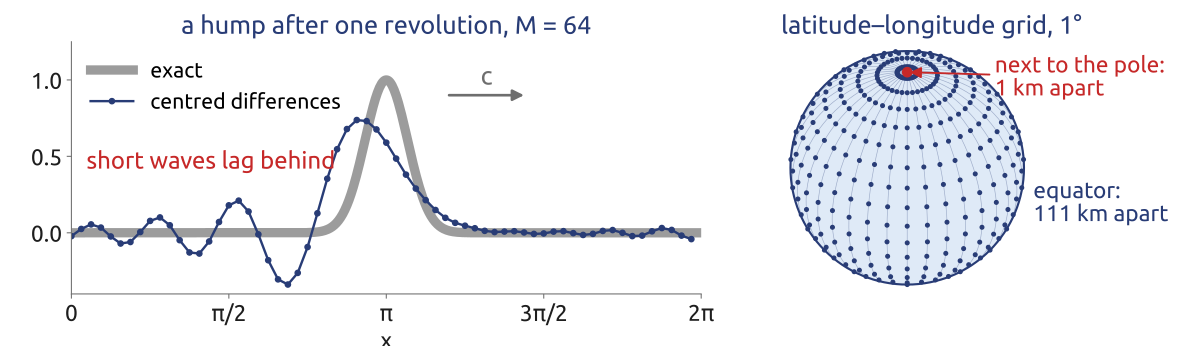
• Advection \(u_t + c\,u_x = 0\) of a narrow hump, once around a periodic domain: centred differences (2nd order), RK4, Courant number 0.1. The short waves lag behind

\(c\): advection speed; Courant number \(c\Delta t/\Delta x\): small, so the error is that of \(\partial_x\)

• A latitude–longitude grid: 111 km between points at the equator, 1 km on the row next to the pole, \(89.5^\circ\)N (CFL)

Today: global waves instead of neighbours. Exact derivatives? No pole problem?

(Durran 2010, Sect. 3.3, 6.4.2; Williamson 2007)

Ask first: what went wrong with the hump? (Short waves lag: dispersion, lecture 5.) Pole: 1° grid (points at the cell centres), 111 km at the equator, 19 km at 80°N, 1 km at 89.5°N: a time step 100 times shorter. Can be skipped if the previous slide was enough.

Von Neumann’s trick (1950)

• ENIAC: finite differences on a flat map, 19 × 16 points
• Each step: \((\delta_x^2 + \delta_y^2)\,\partial_t\psi = -J(\psi, \zeta + f)\), zero on the edges
• Von Neumann: discrete sines are its eigenvectors

\[\begin{aligned} &(\delta_x^2 + \delta_y^2)\Big[\sin\frac{p\pi i}{P}\,\sin\frac{q\pi j}{Q}\Big]\\ &\quad = -\frac{4}{\Delta s^2}\Big[\sin^2\frac{p\pi}{2P} + \sin^2\frac{q\pi}{2Q}\Big]\,\sin\frac{p\pi i}{P}\,\sin\frac{q\pi j}{Q} \end{aligned}\]

\(\delta_x^2\): centred second difference; \(\Delta s\): grid interval; \(i \le P = 18\), \(j \le Q = 15\): grid indices; \(p\), \(q\): mode numbers

• Four sine sums and one division per coefficient: exact for the grid’s Poisson problem

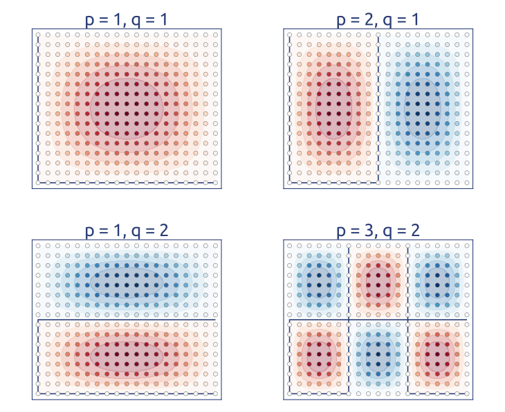
Four discrete sines on the ENIAC grid (19 × 16 points, 736 km apart at the pole).

In a basis of eigenvectors of the discrete Laplacian, the Poisson problem is a division

(Charney et al. 1950; Platzman 1979, 310; Lynch 2008, appendix A; Durran 2010, Sect. 3.1)

Ask first: which step of the 1950 forecast cost the most? (The Poisson solve.) The map: polar stereographic, map factor m = 2/(1 + sin φ), ∇²_globe = m² ∇²_map; in fact solved for the height z (ψ = gz/f₀ in Lynch’s re-creation). Boundary heights held fixed: zero tendency on the edges, so sines fit. The eigenvalue is the finite-difference modified wavenumber squared: for long waves −[(pπ/L_x)² + (qπ/L_y)²], smaller for short ones. Not a spectral model: the first is Silberman (1954). Von Neumann chose this direct method because of the ENIAC’s limits (Platzman); Lynch’s re-creation uses the same method.

Global or local?

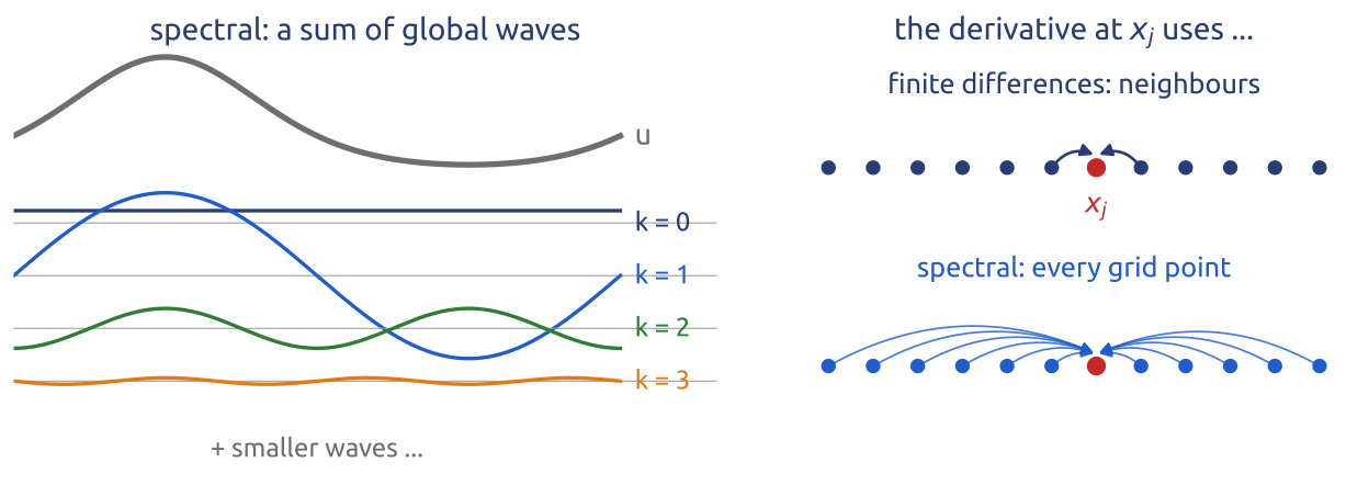
• Spectral: the whole field is a sum of global waves, \(u(x) = \sum_k \hat u_k\,e^{ikx}\)

• Finite differences: a local polynomial through the neighbours

Spectral methods expand the whole field in global waves; finite differences use neighbours

(Durran 2010, Sect. 6.2; Fornberg 1996)

Finite differences: lecture 5. Left: exp(sin x) − 1 and its first waves (from the FFT). Every wave spans the domain: a change at one point changes all coefficients. Right: the derivative at x_j uses two points (FD2) or all (spectral).

Spectral derivative (1/3): interpolate

\(M\) points \(x_j = j\,\Delta x\) on a periodic interval of length \(2\pi\):

\[\begin{aligned} \hat u_k &= \frac{1}{M}\sum_{j=0}^{M-1} u_j\,e^{-ikx_j}\\ u_j &= \sum_{k=-M/2+1}^{M/2}\hat u_k\,e^{ikx_j} \end{aligned}\]

\(u_j\): grid values; \(\hat u_k\): wave coefficients; \(k\): wavenumber

• The sum of waves passes through every grid value: we know \(u\) between the points too
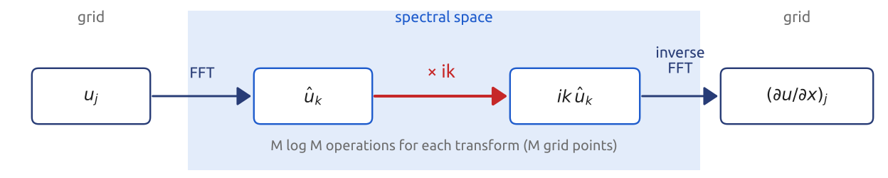
• The FFT computes all \(\hat u_k\) in \(M\log M\) operations

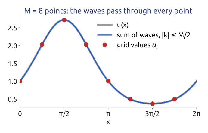
\(M\) grid values and \(M\) wave coefficients carry the same information: the FFT goes back and forth

(Durran 2010, Sect. 6.2; Fornberg 1996)

The discrete Fourier transform and its inverse: M values ↔︎ M coefficients. The wave k = M/2 is (−1)^j on the grid (half of it at +M/2, half at −M/2 for the interpolant). numpy: fft returns M û_k. Notation of the lecture: M grid points, N the largest kept wavenumber (the truncation, as TN on the sphere).

Spectral derivative (2/3): differentiate

Each wave has an exact derivative:

\[\begin{aligned} \frac{d}{dx}\,e^{ikx} &= {\color{#1f5ccc} ik}\,e^{ikx}\\ \Big(\frac{\partial u}{\partial x}\Big)_j &= \sum_k {\color{#1f5ccc} ik}\,\hat u_k\,e^{ikx_j} \end{aligned}\]

• Differentiation = multiply each coefficient by \(ik\)
• The wave \(k = M/2\): derivative set to zero (\((-1)^j\) has no slope at the points)

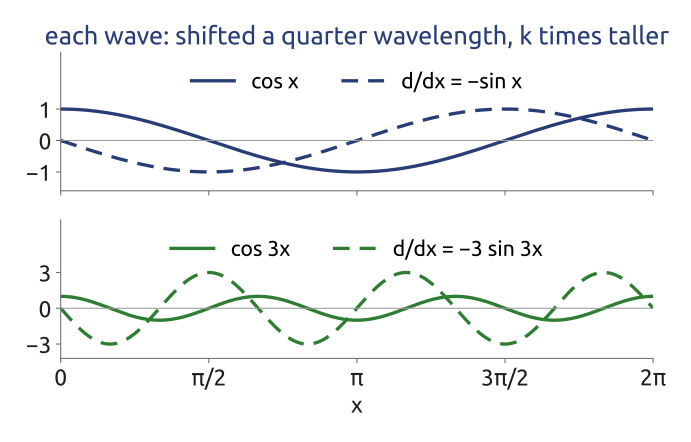
In spectral space, \(\partial_x\) is a multiplication by \(ik\), and \(\nabla^2\) by \(-k^2\)

(Durran 2010, Sect. 6.2)

On the board: d/dx of the interpolant. A derivative turns each wave a quarter wavelength and multiplies it by k. Second derivative: −k².

Spectral derivative (3/3): all waves exact

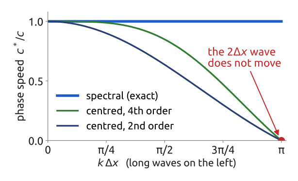
• Centred differences: \(\omega = c\sin(k\Delta x)/\Delta x\), so \(c^*/c = \sin(k\Delta x)/(k\Delta x) < 1\): short waves too slow, the \(2\Delta x\) wave stuck
• Spectral: \(\omega = ck\), \(c^*/c = 1\) for all \(|k| < M/2\)

Advection \(u_t + c\,u_x = 0\), wave \(e^{i(kx-\omega t)}\); \(c^* = \omega/k\): numerical phase speed

The spectral derivative is exact for every wave the grid can carry

(Durran 2010, Sects. 3.3.1 and 6.2.1)

Phase speed c*/c of the centred difference: lecture 5. Ask first: which waves does the centred difference treat worst? (The shortest: 2Δx not at all.) 4th order: (8 sin θ − sin 2θ)/6, better but still bends down.

How fast does the error fall?

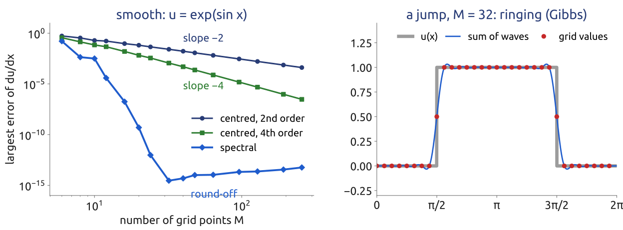
• Smooth fields: the error falls faster than any power of \(\Delta x\) (spectral accuracy); round-off with \(M \approx 32\) points

• Jumps (fronts, coastlines): ringing (Gibbs), slow convergence everywhere

Spectral accuracy for smooth fields; ringing at jumps

(Durran 2010, Sect. 6.2.1; Fornberg 1996)

M = 32: FD2 3e-2, FD4 1e-3, spectral 3e-15. Why: for an analytic periodic function the coefficients fall like e^{-αk}; the error is the first neglected coefficients. With a jump they fall like 1/k.

Advection without numerical dispersion

Advection, \(\partial_t u + c\,\partial_x u = 0\). In spectral space, one ODE per wave:

\[\frac{d\hat u_k}{dt} = -ic{\color{#1f5ccc}k}\,\hat u_k \;\Rightarrow\; \hat u_k = \hat u_k(0)\,e^{-ickt}\]

\(c\): advection speed; \(\hat u_k\): coefficient of the wave \(e^{ikx}\)

• Every wave moves at exactly \(c\); only the time step adds errors

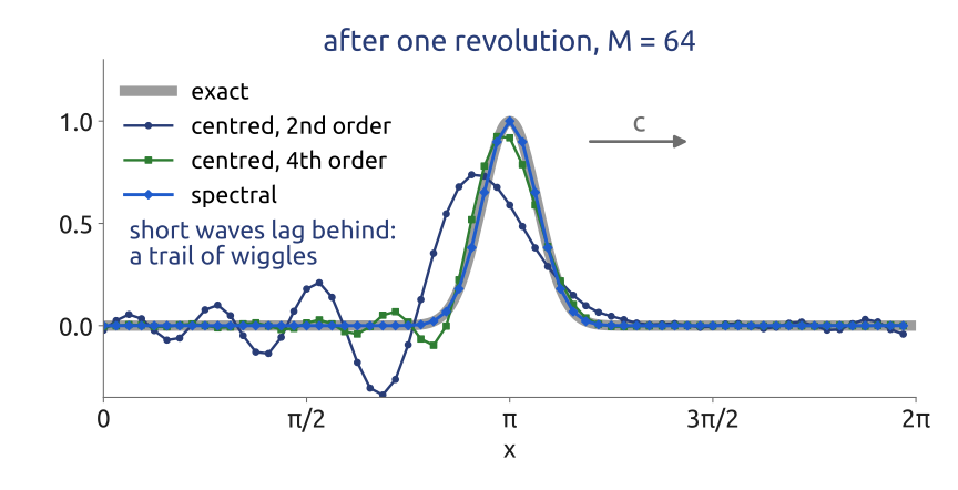
Spectral advection keeps the shape: no numerical dispersion in space

(Durran 2010, Sect. 6.2.1; Williamson 2007)

Advection with grid schemes: lecture 5. Ask first: after one revolution, where will the errors of the centred schemes be: in front or behind? (Behind: short waves lag.) Same RK4 step (Courant 0.1) for all; spectral error 6e-6.

Notebook Fourier spectral methods

Notebook 07a (open in Colab · download): Fourier spectral derivatives, advection and aliasing, on a computer.

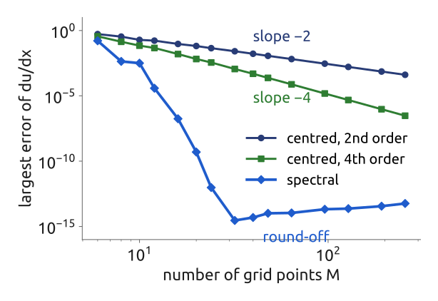
What section 2 should give: slopes −2 and −4, and the spectral drop to round-off

1. The discrete Fourier transform: how fast do the coefficients fall?
2. The spectral derivative against FD2 and FD4: predict the slopes; the second derivative, a kink ❗ 2
3. Advection of a hump, 1 and 10 revolutions; the largest stable time step
4. Products and aliasing: \(u^2\) on 8 points, Burgers with and without the 2/3 rule ❗ 4 (after the next slides)

Predict, run, explain: write down what you expect before each run

A few lines of numpy: an FFT, a multiplication by \(ik\), an inverse FFT

(Durran 2010, Ch. 6; Fornberg 1996)

In class, 25 min: sections 1 to 3 now; section 4 (aliasing) after the 2/3 rule, with the first in-class exercise. Exercise 2: the second derivative, and a field with a kink.

What the notebook showed

Error of \(\partial_x u\), \(u = e^{\sin x}\), \(M = 32\) points:

centred, 2nd order	\(2.6\times10^{-2}\)
centred, 4th order	\(1.1\times10^{-3}\)
spectral	\(2.9\times10^{-15}\)

• The price: Courant number below ~0.9 instead of ~2.8 (RK4): the shortest waves move at full speed

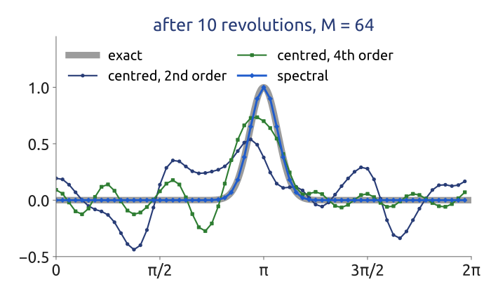
The hump after 10 revolutions: errors 0.65, 0.36 and \(6\times10^{-5}\).

For smooth fields, a few waves do the work of many grid points

(Durran 2010, Sect. 6.2)

Numbers from figures/src/spectral-convergence.py and spectral-advection.py (Courant 0.1; the notebook uses 0.2). A kink (|sin x|): spectral error away from the kink only ~1/M: a defect spreads over the whole domain.

Products (1/3): two waves make new waves

\[\begin{aligned} e^{ikx}\,e^{ilx} &= e^{i(k+l)x}\\ u\,v &= \sum_k \Big({\color{#1f5ccc}\sum_l \hat u_l\,\hat v_{k-l}}\Big)\,e^{ikx} \end{aligned}\]

\(k\), \(l\): wavenumbers; \(u = \sum_l \hat u_l\,e^{ilx}\), \(v = \sum_l \hat v_l\,e^{ilx}\): the waves \(l\) and \(k - l\) make the wave \(k\)

• \(\cos 3x\,\cos 4x = \tfrac12\cos x + \tfrac12\cos 7x\): sum and difference waves
• Two fields with waves up to \(N\): their product has waves up to \(2N\)
• In spectral space a product is a convolution (blue): \(N^2\) operations

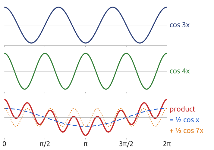
A product of waves makes sum and difference waves, up to twice the highest wavenumber

(Silberman 1954; Ehrendorfer 2012, Sect. 7.5)

Ask first: cos 3x cos 4x = ? (½ cos x + ½ cos 7x.) Silberman (1954), the first spectral model (barotropic vorticity equation on the sphere), computed the products with interaction coefficients: costly, so spectral models stayed tiny until 1970.

Products (2/3): the transform method

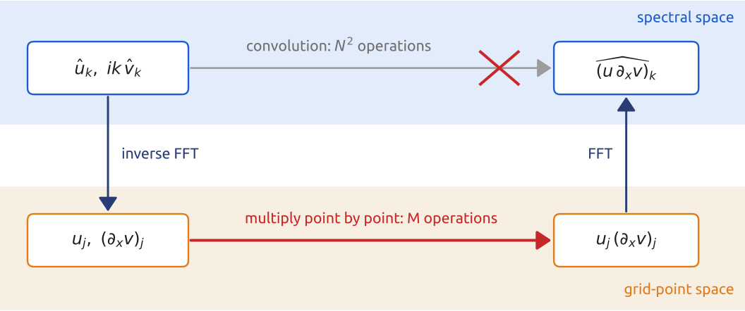
• Orszag (1970), Eliasen, Machenhauer & Rasmussen (1970): derivatives in spectral space, products on the grid

But: the product has waves up to \(2N\), the grid only up to \(M/2\). Where do the others go?

\(N\): the largest kept wavenumber (the truncation); \(M\): the number of grid points, which carry the waves \(|k| \le M/2\)

Derivatives in spectral space, products on the grid: the (spectral) transform method

(Orszag 1970; Eliasen et al. 1970; Ehrendorfer 2012, Sect. 7.7)

Cost: 2 inverse FFTs + M products + 1 FFT, i.e. O(M log M), against N² for the convolution (M ≈ 3N). This made spectral models cost-effective: from the mid-1970s they dominated (Williamson 2007). Names: with as many points as waves (aliased) Durran calls it pseudospectral; the NWP name is “spectral transform”.

Products (3/3): aliasing

\[\begin{aligned} e^{i(k+M)x_j} &= e^{ikx_j}\,e^{2\pi i j} = e^{ikx_j}\\ \tilde u_k = \frac{1}{M}\sum_{j=0}^{M-1} u_j\,e^{-ikx_j} &= {\color{#1f5ccc}\sum_{r} \hat u_{k+rM}} \end{aligned}\]

\(x_j = 2\pi j/M\); \(\hat u_k\): the exact coefficients of \(u(x) = \sum_k \hat u_k e^{ikx}\) (theory); \(\tilde u_k\): the coefficients computed from the \(M\) grid values (numerics), equal to \(\hat u_k\) if \(u\) has no waves beyond \(M/2\); \(r\): any integer

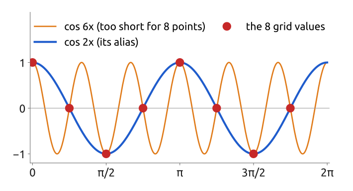
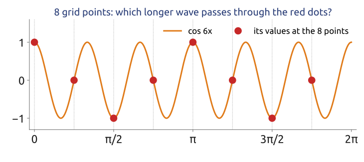
• Figure: \(u = \cos 6x\), \(\hat u_{\pm 6} = \tfrac12\); on 8 points \(\tilde u_{\pm 2} = \tfrac12\): seen as \(\cos 2x\), its alias
• Aliases of a product fall on kept waves: models can blow up (nonlinear instability)

On a grid, a wave too short to be seen pretends to be a longer one

(Durran 2010, Sect. 4.5, 6.3; Ehrendorfer 2012, Sect. 7.9–7.10)

Ask first: on 8 points, which wave looks the same as k = 6? (k = −2, i.e. cos 2x.) Nonlinear instability: Phillips (1959) in a finite-difference model (Durran Sect. 4.5).

The 2/3 rule

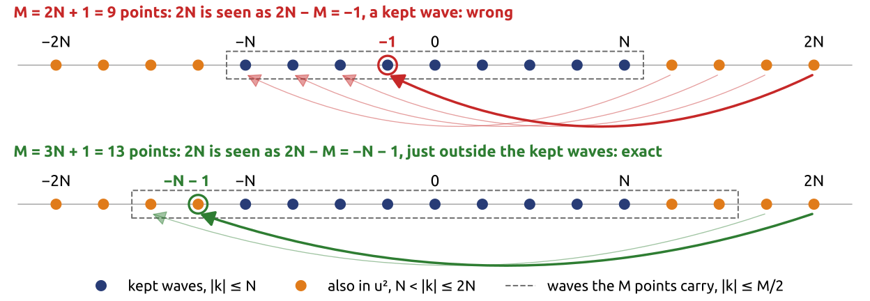
\[2N - M < -N \quad\Longleftrightarrow\quad M \ge 3N + 1\]

\(M\): grid points; \(N\): the largest kept wavenumber (the truncation); \(2N - M\): where the product’s wave \(2N\) lands

• Three points per shortest kept wave: on a given grid, keep the lower two thirds of the waves
• T42: \(3\cdot42 + 1 = 127 \le 128\) longitudes

With three points per shortest kept wave, quadratic products are computed exactly

(Orszag 1971; Durran 2010, Sect. 6.3)

Waves of the product between N and M/2 are on the grid: computed, then dropped by the truncation. Waves beyond M/2 alias to k − M ≤ −N − 1: also dropped. IFS names: linear (2 points), quadratic (3), cubic (4).

In class: aliasing on a small grid

Exercise 1 — Aliasing on a small grid. Take the \(M = 8\) grid points \(x_j = 2\pi j/8\). (a) Show that \(\cos 6x_j = \cos 2x_j\) at every grid point. Which waves look like \(k = 1\) on this grid? (b) \(u = \cos 3x\) is carried by the grid. What does the grid see for \(u^2 = \tfrac12 + \tfrac12\cos 6x\)? (c) A field keeps the waves \(|k| \le N\). How many points \(M\) are needed so that no alias of \(u^2\) falls on a kept wave? Check T42 and its 128 longitudes.

(d) To hand in: cubic products. The same question for \(u^3\). Which fraction of the grid’s waves can be kept? ECMWF’s model uses a “cubic” grid, with four points per shortest wave: why the name?

In notebook 07a (exercise 4): open in Colab · download

(Orszag 1971; Ehrendorfer 2012, Sect. 7.10)

1. k and k ± 8 agree: cos 6x_j = cos(−2x_j) = cos 2x_j; k = 1 looks like 9, −7, 17, … (b) ½ + ½ cos 2x: a wave not in u². (c) alias of 2N is 2N − M < −N: M ≥ 3N + 1; T42: 127 ≤ 128.
2. u³ up to 3N: M ≥ 4N + 1, keep half; the cubic grid computes cubic products exactly. Then section 4 of notebook 7a (10 min): aliasing in u^2, and Burgers’ equation with and without the 2/3 rule.

What the exercise showed

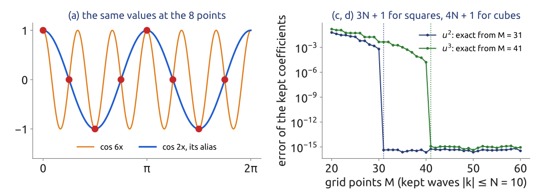
• On 8 points \(k\) and \(k \pm 8\) agree: \(\cos 6x_j = \cos 2x_j\); \(k = 1\) looks like \(9, -7, 17, \dots\)
• \(u^2 = \tfrac12 + \tfrac12\cos 6x\) is seen as \(\tfrac12 + \tfrac12\cos 2x\): a wave not in \(u^2\) at all
• Quadratic products: \(M \ge 3N + 1\) (T42: \(127 \le 128\) longitudes); cubic: \(M \ge 4N + 1\), keep half: the “cubic” grid, four points per shortest wave

Three points per shortest kept wave for squares, four for cubes: then no alias falls on a kept wave

(Orszag 1971; Durran 2010, Sect. 6.3)

The right panel: a random field with |k| <= 10; the error of the kept coefficients drops to round-off at M = 31 (u^2) and M = 41 (u^3).

From the plane to the sphere

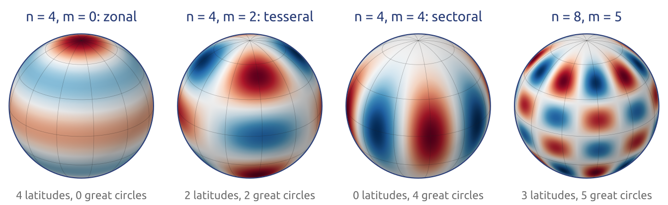
• Spherical harmonics \(Y_n^m = P_n^m(\sin\varphi)\,e^{im\lambda}\): Fourier in longitude, Legendre functions in latitude

• \(n\) = total wavenumber (the scale), \(m\) = zonal wavenumber; smooth at the poles: no pole problem

\(\varphi\): latitude; \(\lambda\): longitude; \(P_n^m\): associated Legendre function, normalised as in the IFS (no \((-1)^m\) factor)

Spherical harmonics are the waves of the sphere

(Ehrendorfer 2012, Sect. 7.11 and App. B.1; ECMWF 2026, Sect. 2.2.4; Durran 2010, Sect. 6.4)

Symbols as in Ehrendorfer and the IFS; Durran writes \(Y_{m,n}\) (order first), the same function with another normalisation. Normalisation: (1/2) int_{-1}^{1} (P_n^m)2 dmu = 1, mu = sin(lat); P_n^{-m} = P_n^m, so a real field has zeta_n^{-m} = conj(zeta_n^m) (Ehrendorfer App. B.1). Ask first: how many nodal lines has Y_4^2? (n = 4: 2 latitudes and 2 great circles.) Fourier in latitude fails: the sphere is not periodic in latitude, and lat-lon grids crowd at the poles.

On the sphere (1/3): the Poisson problem

\[\frac{\partial\zeta}{\partial t} + J(\psi, \zeta + f) = 0, \qquad \zeta = \nabla^2\psi\]

\(J(\psi, q) = \mathbf u\cdot\nabla q\), with \(u = -\frac{1}{a}\frac{\partial\psi}{\partial\varphi}\), \(v = \frac{1}{a\cos\varphi}\frac{\partial\psi}{\partial\lambda}\); \(f = 2\Omega\sin\varphi\): Coriolis parameter; \(\Omega\): rotation rate of the Earth

\(\nabla^2\) is the spherical Laplacian; spherical harmonics are its eigenfunctions:

\[\begin{aligned} \nabla^2 &= \frac{1}{a^2\cos\varphi}\frac{\partial}{\partial\varphi}\Big(\cos\varphi\,\frac{\partial}{\partial\varphi}\Big) + \frac{1}{a^2\cos^2\varphi}\frac{\partial^2}{\partial\lambda^2}\\ \nabla^2 Y_n^m &= -\frac{n(n+1)}{a^2}\,Y_n^m\\ \psi_n^m &= {\color{#1f5ccc} -\frac{a^2}{n(n+1)}}\,\zeta_n^m \quad (n \ge 1) \end{aligned}\]

\(a\): radius of the Earth; \(\lambda\): longitude; \(\varphi\): latitude; \(\psi_n^m\), \(\zeta_n^m\): coefficients of \(Y_n^m\)

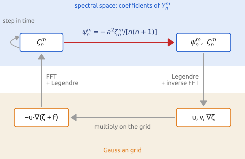
The ENIAC’s Poisson problem on the sphere: a division, as with von Neumann’s sines

(Ehrendorfer 2012, Sect. 7.14; ECMWF 2026, Sect. 2.2.4)

Only n appears in the eigenvalue: m sets the orientation, not the scale. Wavelength about 2πa/n: T42, shortest wave ~950 km; T1279, ~31 km.

On the sphere (2/3): to the grid and back

Inverse: \(u\), \(v\), \(\nabla\zeta\) on the Gaussian grid. Direct: an FFT on each latitude circle, then a Legendre transform by Gaussian quadrature:

\[X_n^m = \sum_{j=1}^{N_{lat}} {\color{#1f5ccc} w_j}\,X_m(\mu_j)\,P_n^m(\mu_j)\]

\(X_m(\mu_j)\): Fourier coefficient on the latitude circle \(\mu_j\); \(\sum_j w_j = 1\)

• \(\mu_j = \sin\varphi_j\): the roots of the Legendre polynomial \(P_{N_{lat}}\) (the Gaussian latitudes), \(w_j\) their weights
• Exact for polynomials in \(\mu\) of degree \(\le 2N_{lat} - 1\)

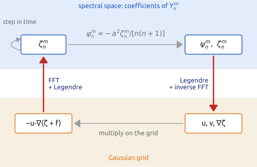
To the grid by inverse transforms; back by an FFT on each latitude and a Gaussian quadrature

(ECMWF 2026, Sect. 2.2.4; Ehrendorfer 2012, Sect. 7.11)

Derivatives on the way: d/dλ → im; cos φ d/dφ via a recursion of the Legendre functions (exact). U = u cos φ, V = v cos φ are smooth at the poles (notebook 7c).

On the sphere (3/3): one time step

On the grid, the product; back to coefficients; step each one in time, with a little diffusion:

\[\frac{d\zeta_n^m}{dt} = -\Big[\mathbf u\cdot\nabla(\zeta + f)\Big]_n^m - \nu_4\Big(\frac{n(n+1)}{a^2}\Big)^2\zeta_n^m\]

\(\nu_4\): coefficient of the \(\nabla^4\) hyperdiffusion; \([\,\cdot\,]_n^m\): coefficient of \(Y_n^m\)

• Linear operators: numbers in spectral space
• Products: on the grid

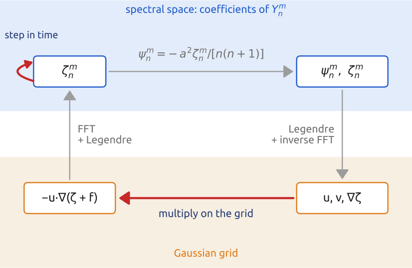
The whole sphere: linear terms in spectral space, products on the grid

(Orszag 1970; Ehrendorfer 2012, Sect. 7.14)

The ∇⁴ diffusion: also a number per coefficient. Time stepping: leapfrog or RK4 (notebook: RK4).

Triangular truncation and the Gaussian grid

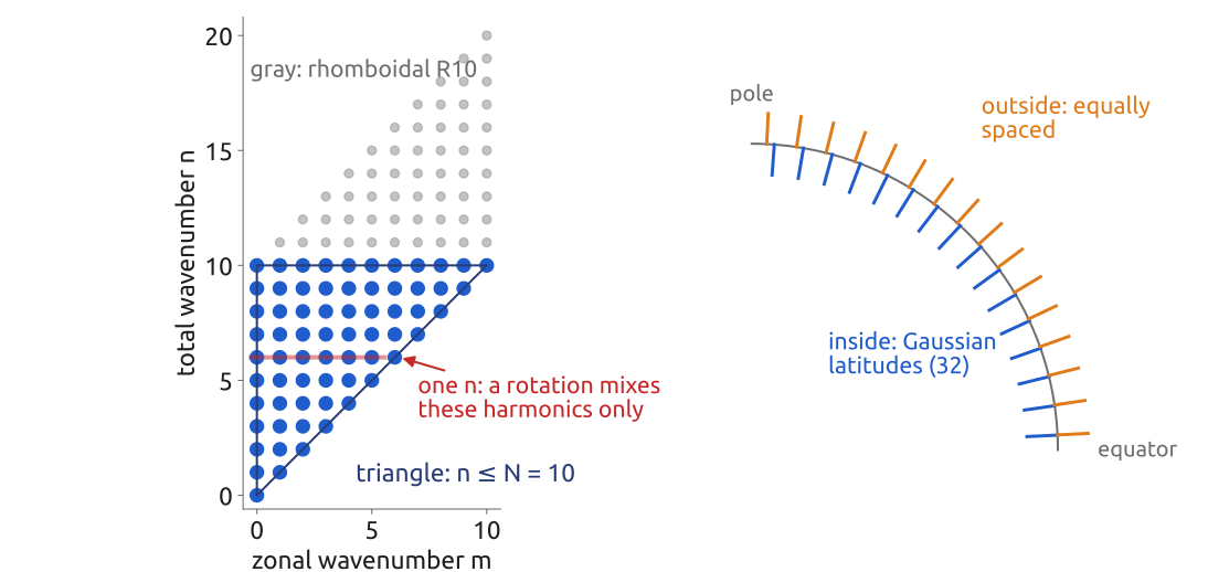
• Keep \(0 \le |m| \le n \le N\): triangular truncation \(N\) (called T\(N\)). A rotation mixes the \(m\) of one \(n\): the same resolution in every direction
• Quadratic grid: \(N_{lat} \ge (3N+1)/2\) Gaussian latitudes, \(3N+1\) longitudes. T42 (\(N = 42\)): 64 × 128
• Shortest wave \(2\pi a/N\): T42 ≈ 950 km

The truncation \(N\) sets the resolution; the grid only has to compute the products exactly

(Ehrendorfer 2012, Sect. 7.11–7.12; Durran 2010, Sect. 6.4.1)

Ask first: why a triangle, not a square (m ≤ N, n − m ≤ N: rhomboidal)? (Isotropy: n is the scale.) Gaussian latitudes are almost equally spaced, a little closer near the poles.

In class: Rossby–Haurwitz waves

Exercise 2 — Rossby–Haurwitz waves. On the sphere, the barotropic vorticity equation linearized about rest is \(\partial_t\nabla^2\psi + (2\Omega/a^2)\,\partial_\lambda\psi = 0\). Take \(\psi = A\,P_n^m(\sin\varphi)\cos(m\lambda - \sigma t)\). (a) With \(\nabla^2 Y_n^m = -n(n+1)Y_n^m/a^2\), find \(\sigma\) and the angular speed \(\sigma/m\) of the pattern. East or west? (b) How many days does it take to go once round the Earth for \(n = 1, 2, 5\)? What is special about \(n = 1\)?

(c) To hand in: a stationary wave. Add an eastward wind in solid-body rotation, \(u = \omega a\cos\varphi\) (the air turns a little faster than the Earth). The pattern then turns at \(\omega - 2(\Omega + \omega)/[n(n+1)]\). Which \(\omega\) makes the wave \(n = 5\) stationary? What is \(u\) at the equator and at \(45^\circ\)N?

In notebook 07c (exercise 1): open in Colab · download

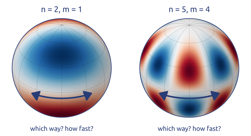
(Haurwitz 1940; Williamson et al. 1992)

1. Substituting, the common factor sin(mλ − σt) leaves −n(n+1)σ/a² − 2Ωm/a² = 0, which gives σ = −2Ωm/[n(n+1)]: angular speed −2Ω/[n(n+1)], westward; depends on n only.
2. period πn(n+1)/Ω: n = 1: 0.997 d (fixed in space: a tilted solid-body rotation), n = 2: 3.0 d, n = 5: 15 d.
3. ω = 2Ω/(n(n+1) − 2) = Ω/14: u = 33 m/s at the equator, 23 m/s at 45°N (Rossby’s stationary waves).

What the exercise showed

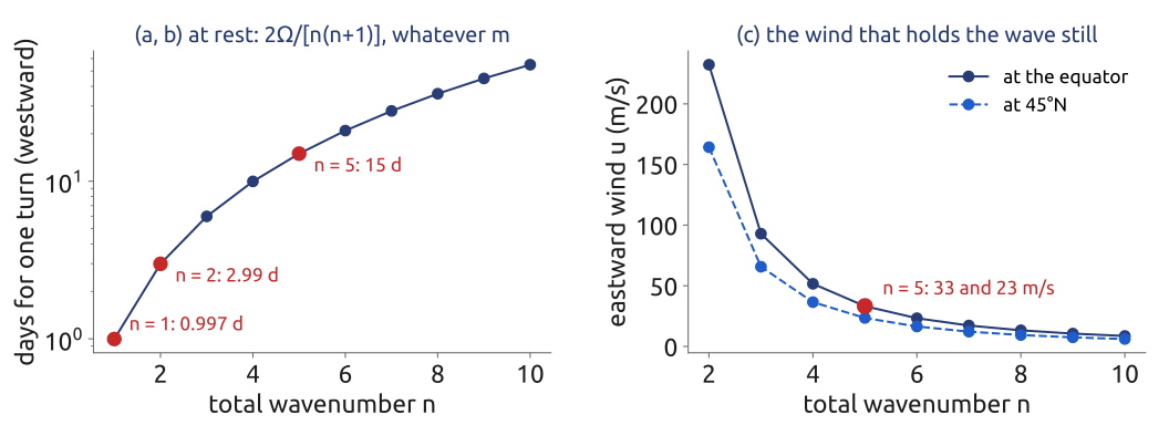
• \(\nabla^2 Y_n^m = -n(n+1)Y_n^m/a^2\) leaves \(-n(n+1)\sigma - 2\Omega m = 0\): \(\sigma/m = -2\Omega/[n(n+1)]\), westward, the same for every \(m\) of one \(n\); the largest scales are the fastest
• Once round the Earth: \(n = 1\) in 1 day (fixed in space: a tilted solid-body rotation), \(n = 2\) in 3 days, \(n = 5\) in 15
• An eastward wind of 33 m/s at the equator (23 m/s at 45°N) holds the wave \(n = 5\) still: Rossby’s stationary waves

On the sphere the Rossby waves are spherical harmonics, and their speed depends on \(n\) only

(Haurwitz 1940; Williamson et al. 1992)

omega = 2 Omega/(n(n+1) - 2) = Omega/14 for n = 5. The model of 7c reproduces the speeds to five digits.

Notebook Vorticity: plane and sphere

Notebooks 07b (open in Colab · download) and 07c (open in Colab · download): the barotropic vorticity equation on a plane and on the sphere.

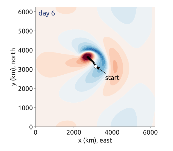
Expected in 07b: the cyclone drifts north-west

• 07b, the β-plane: the pseudo-spectral model; Rossby waves against \(\omega = -\beta k/(k^2 + l^2)\); a cyclone: predict where it goes; ❗ 1 (the dispersion relation); two-dimensional turbulence (at home)
• 07c, the sphere: the transform in numpy (Gaussian latitudes, Legendre functions); Rossby–Haurwitz waves ❗ 1; an unstable jet (at home)

Predict, run, explain: model against exact speeds; the drift of the cyclone

The same model, plane or sphere: derivatives in waves, products on the grid

(Williamson et al. 1992; Galewsky et al. 2004)

In class, 25 min: 07b sections 3–4 and 07c sections 2–4 (with exercise 1). At home: 07b section 5 (turbulence) and 07c section 5 (the jet, exercise 2, resolution).

What the notebooks showed

• Rossby waves: model frequency = theory to all printed digits
• The cyclone drifts north-west ~1 m/s (β drift), leaving Rossby waves behind
• Rossby–Haurwitz wave: 122° east in 10 days, error \(10^{-8}\); westward at rest, \(2\Omega/[n(n+1)]\)
• The jet: a tiny bump grows into breaking waves in 4–6 days; T42 and T63 disagree by day 6. Laptop: seconds per forecast day; ENIAC: a day per day

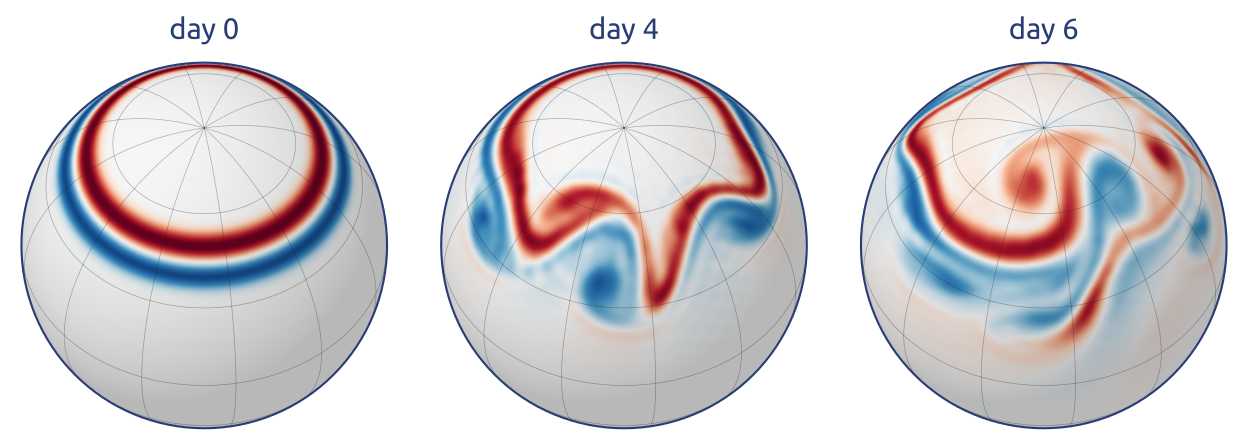
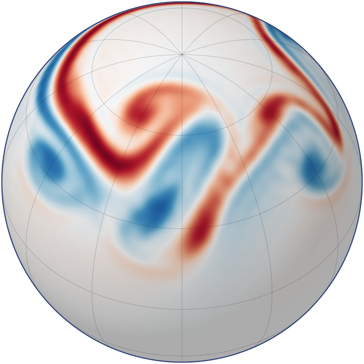
A barotropically unstable jet (80 m/s at 45°N), T63, notebook 7c.

A spectral barotropic vorticity model of the whole sphere, in sixty lines of numpy

(Galewsky et al. 2004; Williamson et al. 1992)

The jet: Galewsky et al. (2004) shape, for the vorticity equation (no height field). The bump sets where the waves appear: small initial errors grow, and so do resolution differences (07c exercise 2). Next: the full equations bring gravity waves.

Semi-implicit (1/2): the gravity-wave limit

• The barotropic vorticity equation has no gravity waves; shallow water and the full equations do. Linear, no rotation, with the divergence \(\delta = \nabla\cdot\mathbf u\):

\[\frac{\partial\delta}{\partial t} = -g\nabla^2 \eta, \qquad \frac{\partial \eta}{\partial t} = -H\delta\]

\(\eta\): height perturbation; \(H\): mean depth; \(g\): gravity

• Waves at \(\sqrt{gH} \approx 300\) m/s, ten times the wind: an explicit step must follow them (CFL)
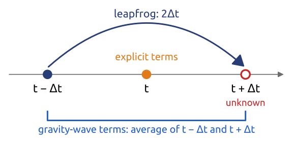
• Robert (1969): these terms implicit (average of \(t - \Delta t\) and \(t + \Delta t\)), the rest explicit

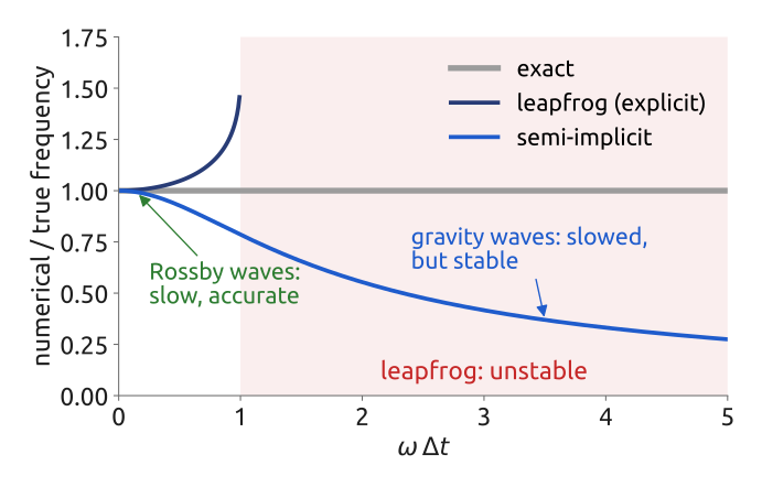
Averaged gravity-wave terms are stable for any \(\Delta t\): fast waves slowed, slow waves accurate

(Staniforth 1997; Durran 2010, Sect. 8.2)

Gravity waves: lecture 3. Ask first: what limits the time step of an explicit global model? (The fastest gravity waves, not the wind.) Test equation dF/dt = iωF: leapfrog sin(ω_num Δt) = ωΔt (unstable for ωΔt > 1); averaged tan(ω_num Δt) = ωΔt. The idea came after a seminar on implicit methods by G. I. Marchuk (Staniforth 1997).

Semi-implicit (2/2): Helmholtz, a division

Leapfrog with the gravity-wave terms averaged (\(\pm\): \(t \pm \Delta t\); dots: explicit terms):

\[\begin{aligned} \delta^{+} &= \delta^{-} - g\Delta t\,\nabla^2\big(\eta^{+} + \eta^{-}\big) + \dots\\ \eta^{+} &= \eta^{-} - H\Delta t\,\big(\delta^{+} + \delta^{-}\big) + \dots \end{aligned}\]

Put \(\eta^{+}\) into the first equation: a Helmholtz problem (below)

• Grid models: an elliptic problem on the whole globe, every step (iterative solvers)
• Spectral: one division per coefficient, “negligible for a spectral model”
• Many levels: a small matrix per \(n\) couples them; its eigenvectors are the vertical modes

\[\Big(1 - gH\Delta t^2\,\nabla^2\Big)\,\delta^{+} = R \quad\Rightarrow\quad \delta_n^{m,+} = \frac{R_n^m}{1 + gH\Delta t^2\,{\color{#1f5ccc} n(n+1)/a^2}}\]

\(R\): everything known at \(t\) and \(t - \Delta t\); \(R_n^m\), \(\delta_n^{m,+}\): coefficients of \(Y_n^m\)

Semi-implicit: one Helmholtz problem per step, a division in spectral space

(Staniforth 1997, 35; ECMWF 2026, Sect. 2.2.7; Durran 2010, Sect. 8.2.3)

Vertical modes: lecture 4, appendix. On the board: eliminate η⁺; the factor Δt² comes from the two averages over 2Δt. IFS: Eq. (2.50) of the documentation, [I + n(n+1)/a² Γ] D⁺ = D̃ for each (m, n), Γ an NLEV × NLEV matrix.

The grids of the IFS

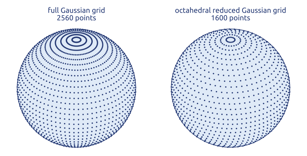
• Near the poles a harmonic of large \(m\) is tiny: points can be dropped there. Reduced Gaussian grid since 1991
• Octahedral since March 2016: 20 points next to the pole, 4 more per latitude
• Cubic grid: 4 points per shortest wave. TCo1279 = 1280 latitudes per hemisphere, 6.6 million points per level, about 9 km

The truncation fixes the resolution; the grid only needs enough points for the products

(ECMWF 2026, Sect. 2.2.5–2.2.6; Malardel et al. 2016)

Ask first: why can a spectral model drop points near the poles, and a lat-lon finite-difference model not? (The truncation already removes the short waves there; no CFL limit from the grid.) Octahedral: 22% cheaper than the original reduced grid; FFTW allows any number of points per circle.

IFS today

Resolution	TCo1279: ~9 km, 137 levels up to 0.01 hPa
Spectral	wind, temperature, surface pressure; moisture and tracers on the grid
Advection	semi-Lagrangian: departure points and interpolation
Time step	semi-implicit, about 7 min
Ensemble	50 + 1 members at 9 km
History	ECMWF’s first spectral model in operations: April 1983

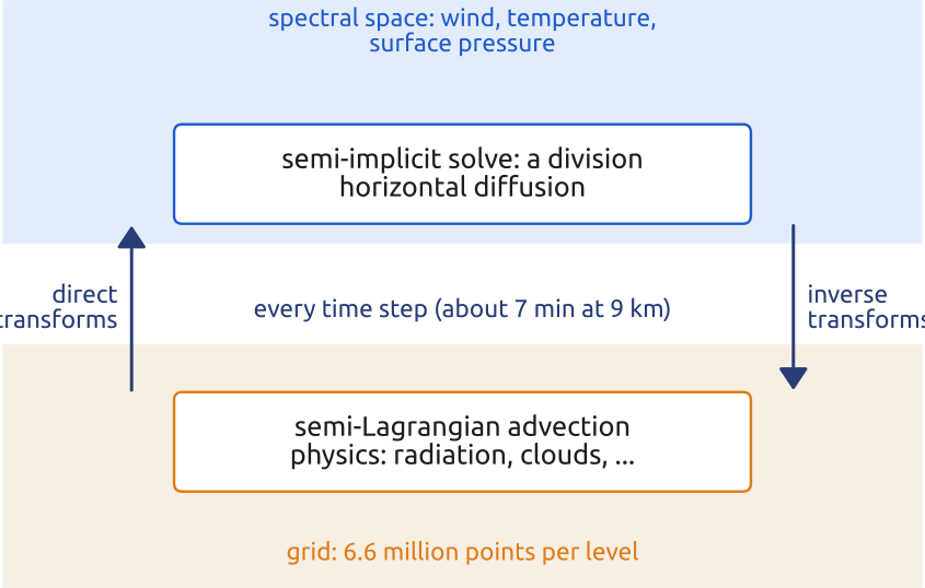
The IFS: linear terms in spectral space, advection and physics on the grid, transforms every step

(ECMWF 2026; Malardel et al. 2016) · Configuration: confluence.ecmwf.int: Model information (Cy50r1)

Cycle 50r1, operational 12 May 2026. Semi-Lagrangian: follow the air back one step and interpolate: stable for long steps (lecture 9). Time step: 400 s in Malardel et al. (2016).

The cost of the transforms

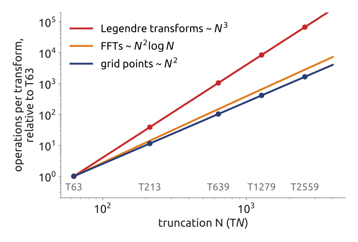
Operations for one transform of one field (one time step) on a quadratic Gaussian grid, each curve divided by its value at T63: how fast each part grows, not which costs most.

• Legendre transforms: \(N^2/2\) coefficients × \(1.5\,N\) latitudes: \(\sim N^3\); FFTs \(\sim N^2\log N\); grid points \(\sim N^2\)
• Double the resolution: grid ×4, Legendre ×8 (and the time step halves)
• Every coefficient needs every grid point: global communication on the whole supercomputer, every step
• Fast Legendre transforms (Wedi et al. 2013) reduce the cost, not the communication

Spectral transforms are global: their cost and communication grow faster than the grid

(Williamson 2007; Wedi et al. 2013)

Ask first: double the resolution: how much more work per time step? (Grid ×4, Legendre ×8.) Bridge to lectures 8–9: methods that only talk to neighbours (finite volumes, finite elements).

Spectral models today

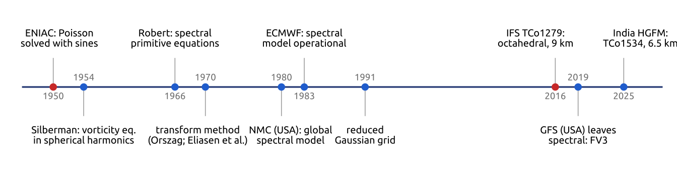
• IFS (ECMWF): TCo1279, 9 km
• ARPEGE (Météo-France): a stretched sphere, ~7 km over France
• GSM (JMA, Japan): TQ959, ~13 km

• BAM (CPTEC, Brazil): TQ0666, ~20 km
• HGFM (IITM, India): TCo1534, ~6.5 km
• YHGSM (NUDT, China): spectral, semi-Lagrangian
• GFS (NOAA, USA): spectral 1980–2019, then finite volumes (FV3)

• AROME (Météo-France): limited area, Fourier in \(x\) and \(y\), 1.3 km
• EC-Earth3 (European climate model, 27 partners, Italian institutes among them): the IFS at T255, ~80 km

Spectral models are not over: new ones keep coming, at kilometre scales

(Météo-France 2016; Yonehara et al. 2025; Figueroa et al. 2016; Krishna et al. 2025; Jiang et al. 2021; Döscher et al. 2022; Sela 1980) · GFS documentation

Not superseded: India’s newest model (2025) is spectral, at 6.5 km, for monsoon rainfall. ECMWF also develops a finite-volume core (FVM) for the future. ARPEGE: Schmidt’s stretching, T1198c2.2 in 2016 (Courtier and Geleyn 1988). AROME: Météo-France’s limited-area model, 1.3 km (2016 report). JMA: quadratic grid since March 2023. BAM: spectral, Eulerian or semi-Lagrangian, semi-implicit (Figueroa et al. 2016).

A Galerkin method

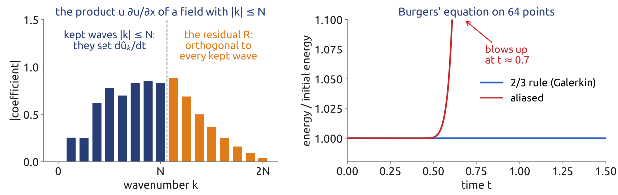
\[R = \frac{\partial u_N}{\partial t} + F(u_N), \quad \int_0^{2\pi}\! R\,e^{-ikx}\,dx = 0 \;\; (|k| \le N)\]

\(u_N = \sum_{|k| \le N}\hat u_k e^{ikx}\): the truncated field; \(F\): the space-derivative terms (here \(u\,\partial_x u\)); \(R\): the residual

• The residual has no part along any kept wave: the transform method with the 2/3 rule is exactly this
• So the energy \(\tfrac12\int u_N^2\,dx\) is conserved: no nonlinear instability
• Finite elements: the same condition, with local functions on any mesh

The spectral method is a Galerkin method with global waves; finite elements use local functions

(Durran 2010, Sects. 6.1 and 6.2.3)

Ask first: why did the aliased run blow up? (The computed product is not the projection of u u_x: energy is not conserved.) Burgers forms a shock at t = 0.54; the Galerkin energy stays constant even then. Next: finite elements, the same Galerkin condition with hats (lecture 8).

Key points

1. Spectral derivative: exact for every resolved wave; spectral accuracy for smooth fields; ringing at jumps
2. Transform method: products on the grid; aliasing; the 2/3 rule (\(3N + 1\) points)
3. Spherical harmonics \(Y_n^m\): \(\nabla^2 Y_n^m = -n(n+1)Y_n^m/a^2\); triangular truncation \(N\) (T\(N\)); Gaussian grid; no pole problem
4. Poisson and Helmholtz problems are divisions: semi-implicit steps are cheap
5. Legendre transforms cost \(\sim N^3\) and need global communication: the scaling limit
6. The IFS: spectral, semi-Lagrangian, semi-implicit, 9 km
7. A Galerkin method: the residual is orthogonal to every kept wave; energy conserved without aliasing

Notebooks 07a (open in Colab · download), 07b (open in Colab · download) and 07c (open in Colab · download): exercise 1 comes back in 07a, exercise 2 in 07c.

Spectral methods: exact derivatives and cheap implicit steps, at the price of global transforms

Reading: (Durran 2010, Ch. 6 and sec. 8.2; Ehrendorfer 2012; Williamson 2007; ECMWF 2026, Sect. 2.2.4)

Next lecture’s warm-up asks about these. Still open: jumps and positivity (fronts, moisture: kept on the grid). Next: local, high order, on any mesh: can a method have all three? The spectral method is a Galerkin method; finite elements do the same with local functions (lecture 8).