Finite elements: from Galerkin to discontinuous Galerkin
Atmosphere and Ocean Dynamics, Lecture 8: notes
Finite elements: local basis functions on any mesh. These notes discuss the weak form and Galerkin’s method with hat functions; continuous and discontinuous Galerkin (DG) methods for advection, with numerical fluxes, a block-diagonal mass matrix, convergence of order \(p + 1\) and the time-step limit; DG in two dimensions with Firedrake; compatible finite elements, the C grid on any mesh, which conserve energy and keep geostrophic balance; and the dynamical cores built on them, Gusto and the Met Office’s LFRic.
1 Why local?
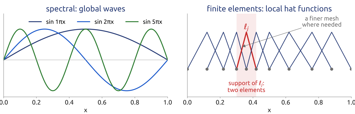
Spectral methods expand the fields in global functions, Fourier waves or spherical harmonics: every coefficient depends on every grid point, and each transform needs a global exchange of data on a parallel computer. Finite-element methods also expand the fields in basis functions, but each basis function is non-zero on a few elements only (its support). The equations for the coefficients then couple only neighbouring elements; the mesh can be unstructured and refined where needed; and inside each element the polynomial degree can be raised for accuracy (Figure 1). The price is a systematic way of deriving equations for the coefficients: the weak form (Durran 2010, sec. 6.5; Marras et al. 2016).
2 Weak form (1/4): multiply and integrate
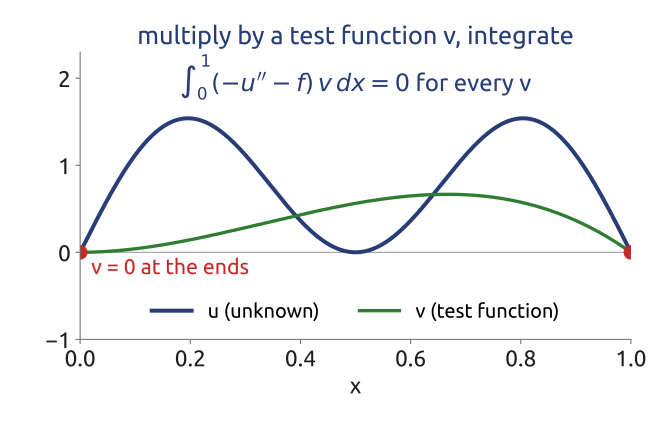
The model problem is the one-dimensional Poisson problem, the one-dimensional version of the Poisson problem that the 1950 forecast solved at every step: \[ -u'' = f \quad\text{on } (0, 1), \qquad u(0) = u(1) = 0 , \] with \(u\) the unknown, \(f\) a given source and a prime the derivative \(d/dx\). Multiply by a test function \(v\) with \(v(0) = v(1) = 0\) and integrate: \(\int_0^1 (-u'' - f)\,v\,dx = 0\). If this holds for every \(v\), the equation holds: take \(v\) concentrated near any point (Figure 2).
3 Weak form (2/4): integrate by parts
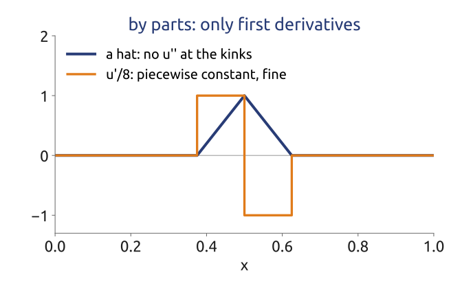
Integration by parts moves one derivative from \(u\) to \(v\): \(-\int_0^1 u''v\,dx = \int_0^1 u'v'\,dx - [u'v]_0^1\), and the boundary term vanishes because \(v = 0\) at the ends. The weak form is: find \(u\) with \(u(0) = u(1) = 0\) such that \[ \int_0^1 u'\,v'\,dx = \int_0^1 f\,v\,dx \qquad \text{for every } v \text{ with } v(0) = v(1) = 0 . \] Only first derivatives appear: a function with kinks, piecewise linear for example, has no second derivative at the kinks, but its first derivative is piecewise constant and the integral makes sense (Figure 3). “For every \(v\)”, however, is infinitely many equations.
Mathematical aside. The natural space is \(H^1_0(0,1)\), the functions with a square-integrable derivative that vanish at the ends. With \(a(u, v) = \int u'v'\,dx\), bounded and coercive on \(H^1_0\) (Poincaré’s inequality), the Lax–Milgram theorem gives a unique weak solution for every \(f\) in \(L^2\).
4 Galerkin (3/4): a finite set of hats
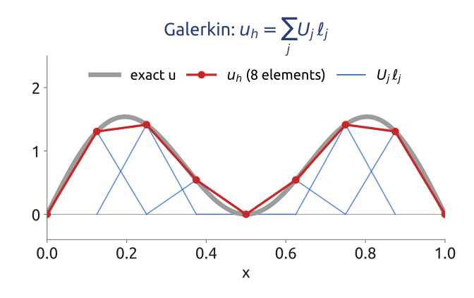
Cut \([0, 1]\) into elements by nodes \(0 = x_0 < x_1 < \dots < x_n = 1\), and let \(\ell_j\) be the hat function of node \(j\), the linear Lagrange function: 1 at \(x_j\), 0 at the other nodes, linear on each element. Look for \(u_h = \sum_{j=1}^{n-1}U_j\ell_j\), with the nodal values \(U_j\) as unknowns, and test with each \(v = \ell_i\): the Galerkin method, with trial and test functions from the same finite space, \[ \sum_j \Big(\int_0^1\ell_i'\ell_j'\,dx\Big)U_j = \int_0^1 f\,\ell_i\,dx, \qquad\text{i.e.}\qquad SU = F , \] with the stiffness matrix \(S\). There is one equation per unknown, and \(S_{ij} \ne 0\) only if \(\ell_i\) and \(\ell_j\) overlap: the matrix is sparse (Figure 4).
Mathematical aside. Galerkin’s method is optimal in the energy norm: \(a(u - u_h, v_h) = 0\) for every \(v_h\) in the finite space (Galerkin orthogonality), and Céa’s lemma gives \(\|u - u_h\|_{H^1} \le C\min_{v_h}\|u - v_h\|_{H^1}\), an error of order \(h\) for hats; with a duality argument, order \(h^2\) in \(L^2\). For this one-dimensional problem with exact load integrals, \(u_h\) is even exact at the nodes.
5 Galerkin (4/4): the matrices
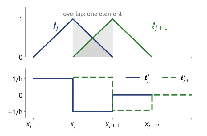
On a uniform mesh of size \(h\), \(\ell_j' = 1/h\) on \([x_{j-1}, x_j]\) and \(-1/h\) on \([x_j, x_{j+1}]\), and only neighbours overlap: \[ S = \frac1h\,\mathrm{tridiag}(-1, 2, -1), \qquad M = \frac h6\,\mathrm{tridiag}(1, 4, 1) , \] with the mass matrix \(M_{ij} = \int\ell_i\ell_j\,dx\), which appears with the time derivative in time-dependent problems, \(\int\partial_t u_h\,\ell_i\,dx = (M\dot U)_i\) (Figure 5). With \(F_j \approx h f(x_j)\), row \(j\) of \(SU = F\) is \((-U_{j-1} + 2U_j - U_{j+1})/h^2 = f(x_j)\): the centred second difference. The difference from finite differences is not this row but what comes with it: any mesh, any degree, and a proof of convergence.
6 Continuous Galerkin for advection
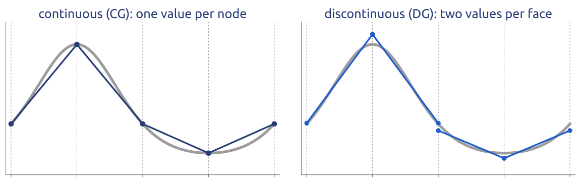
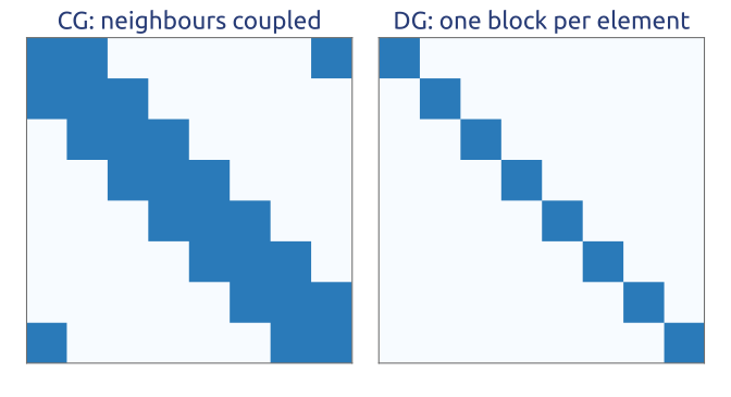
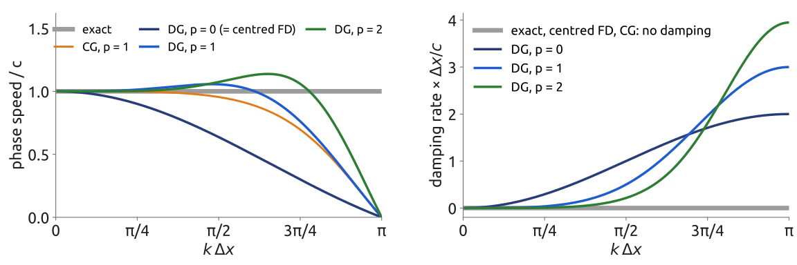
For \(u_t + c\,u_x = 0\) on a periodic interval, the same procedure gives \(M\dot U = -c\,\big[\int\ell_i\,\ell_j'\,dx\big]\,U\), where \(\int\ell_i\,\ell_j'\,dx\) is \((-\tfrac12, 0, \tfrac12)\) on a uniform mesh: \[ \frac{\dot U_{j-1} + 4\dot U_j + \dot U_{j+1}}{6} = -c\,\frac{U_{j+1} - U_{j-1}}{2h} . \] For a wave \(e^{i(kx-\omega t)}\) this gives the numerical frequency \(\omega h/c = 3\sin kh/(2 + \cos kh)\), accurate to fourth order in the phase, better than the centred difference, \(\omega h/c = \sin kh\) (Durran 2010, sec. 3.3.1). But the inverse of the tridiagonal mass matrix couples all unknowns, so each explicit time step needs a linear solve, a sparse global solve in two or three dimensions; and the scheme is centred, with no damping of grid-scale noise (Durran 2010, sec. 6.5.1). Letting the solution jump between elements removes both (Figure 6).
7 DG (1/4): a polynomial in each element
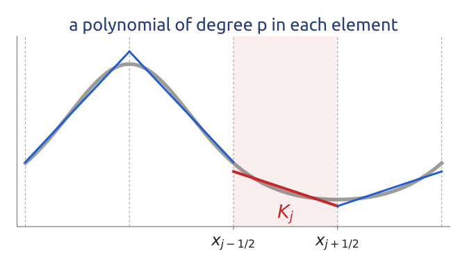
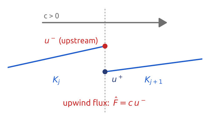
On each element \(K_j = [x_{j-1/2}, x_{j+1/2}]\) the solution is a polynomial of degree \(p\), with no continuity between elements: the broken space \(V_h = \{v : v|_{K_j}\in\mathbb P_p \text{ for every } K_j\}\), with \(\mathbb P_p\) the polynomials of degree at most \(p\) (Durran and Hesthaven & Warburton write \(N\) for the degree, Cockburn \(k\)). Each element has \(p + 1\) unknowns, and at each face \(u_h\) has two values, \(u^-\) from the left element and \(u^+\) from the right one (Figure 7). Reed and Hill introduced the method in 1973 for neutron transport; Cockburn and Shu developed it for conservation laws (Cockburn 2003; Hesthaven and Warburton 2008).
8 DG (2/4): integrate by parts in one element
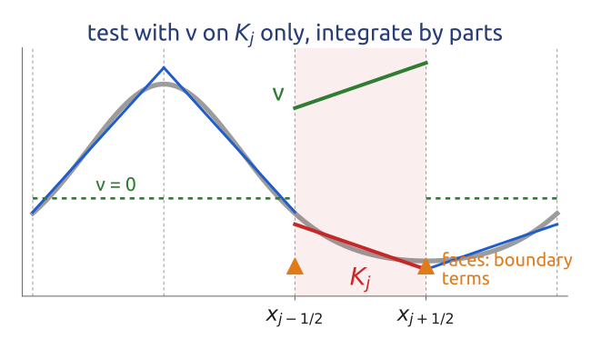
Take a test function \(v\) that lives on \(K_j\) only, multiply, integrate over \(K_j\) and move the derivative to \(v\): \[ \int_{K_j}\partial_t u_h\,v\,dx - \int_{K_j}c\,u_h\,\partial_x v\,dx + \hat F_{j+1/2}\,v(x_{j+1/2}^-) - \hat F_{j-1/2}\,v(x_{j-1/2}^+) = 0 , \] where \(\hat F\) is the numerical flux at a face. The boundary terms are the fluxes through the two faces, and the equations of one element meet those of its neighbours only there: they are local (Figure 8). As in a finite volume, this is the integral form over the element, but with a polynomial instead of a constant, and for every test function of the element (Durran 2010, sec. 6.6; Hesthaven and Warburton 2008).
9 DG (3/4): the numerical flux
At a face \(c\,u\) has two possible values: we choose one flux \(\hat F(u^-, u^+)\), the same for the two elements that share the face, so that what leaves one element enters the other (conservation), and consistent, \(\hat F(u, u) = c\,u\). For \(c > 0\) the upwind flux takes the value from upstream, \(\hat F = c\,u^-\) (Figure 9), the choice of the upwind finite-volume scheme. Other choices are the central flux \(c\,(u^- + u^+)/2\), the Lax–Friedrichs flux and, for systems, approximate Riemann solvers (Cockburn 2003; LeVeque 2002).
10 DG (4/4): local mass matrices
Write \(u_h|_{K_j} = \sum_l U_{j,l}\,P_l\) and take \(v = P_i\), \(i = 0, \dots, p\), with \(P_l\) polynomials of degree at most \(p\), for instance Legendre polynomials. Then \[ M_K\,\frac{dU_j}{dt} = R(U_j, U_{j-1}) , \] with the coefficients \(U_j\) of element \(j\), its mass matrix \(M_K\) and the volume and face terms \(R\). The mass matrix is block diagonal, one small \((p+1)\times(p+1)\) block per element (diagonal with Legendre polynomials), inverted once and for all (Figure 10). Explicit Runge–Kutta methods advance each element with data from its neighbours only: one layer of data exchange on a parallel computer.
11 p = 0: a finite-volume scheme
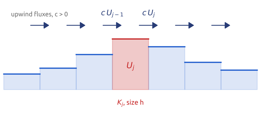
With \(p = 0\), \(u_h = U_j\) on \(K_j\), \(v = 1\) and \(\partial_x v = 0\): \[ h\,\frac{dU_j}{dt} = -\big(c\,U_j - c\,U_{j-1}\big) , \] with \(U_j\) the mean of \(u\) on \(K_j\) and \(h\) the element size: the upwind (donor-cell) finite-volume scheme (Figure 11). Every DG scheme contains this finite-volume balance, since the test function \(v = 1\) on \(K_j\) gives the conservation of the element average (Cockburn 2003; LeVeque 2002).
12 Higher order: a Legendre basis
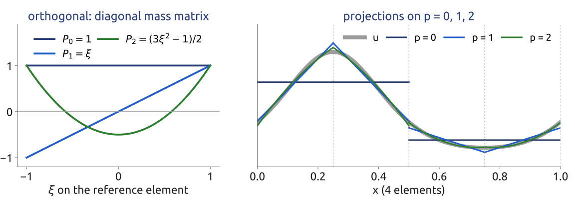
On the reference element \(\xi \in [-1, 1]\), \(x = x_j + h\xi/2\), the Legendre polynomials \(P_l(\xi)\) are orthogonal, \(\int_{K_j}P_iP_l\,dx = \frac{h}{2i+1}\delta_{il}\), so the mass matrix is diagonal. The volume term is \(c\sum_l D_{il}U_{j,l}\) with the derivative matrix \(D_{il} = \int_{-1}^1 P_l P_i'\,d\xi\) (the factors \(h/2\) and \(2/h\) cancel), and at the faces \(P_i(1) = 1\), \(P_i(-1) = (-1)^i\). With the upwind flux the scheme is \[ \frac{dU_{j,i}}{dt} = \frac{2i+1}{h}\Big[c\sum_l D_{il}U_{j,l} - c\,u_j(1) + (-1)^i\,c\,u_{j-1}(1)\Big], \qquad u_j(1) = \sum_l U_{j,l} \] (Hesthaven and Warburton 2008; Durran 2010, sec. 6.6.1). With orthogonal polynomials each element is a tiny spectral method (Figure 12). This is a modal basis; nodal bases, Lagrange polynomials at Gauss–Lobatto points, are also common, and spectral elements are their continuous version.
13 Order p + 1, and the time step
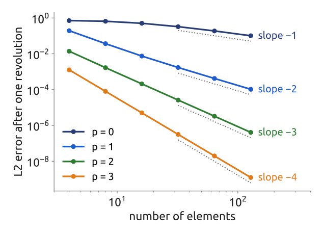
For smooth solutions the DG error with the upwind flux falls like \(h^{p+1}\): slopes 1, 2, 3 and 4 for \(p = 0, \dots, 3\) (Figure 13) (Cockburn 2003). The DG operator is integrated in time with the third-order strong-stability-preserving Runge–Kutta method (SSP-RK3) of Shu and Osher (1988) (the name is due to Gottlieb et al. (2001)). Its largest stable Courant number \(c\Delta t/h\), computed from the eigenvalues of the scheme (next section), is about 1.26 for \(p = 0\), 0.41 for \(p = 1\), 0.21 for \(p = 2\) and 0.13 for \(p = 3\). Cockburn’s von Neumann analysis gives \(c\Delta t/h \le 1/(2p+1)\) for a Runge–Kutta method of order \(p+1\) (Cockburn 2003, sec. 3.3), close to these numbers; for large \(p\) the limit falls like \(p^{-2}\) (Hesthaven and Warburton 2008, sec. 4.8). An element of degree \(p\) holds \(p + 1\) unknowns: it behaves like a grid \(p + 1\) times finer.
14 Dispersion and dissipation
Bloch analysis. For the wave \(e^{ikx}\) the coefficients of neighbouring elements differ by a phase, \(U_{j-1} = e^{-ikh}U_j\), and the semi-discrete scheme becomes \(\dot U_j = A(kh)\,U_j\) with a \((p+1)\times(p+1)\) matrix. One of its eigenvalues, \(\lambda(k)\), approximates the exact \(-ick\): \(-\mathrm{Im}\,\lambda\) is the numerical frequency \(\omega\), with phase speed \(c^* = \omega/k\), and \(-\mathrm{Re}\,\lambda\) the damping. Per unknown, DG with \(p \ge 1\) moves resolved waves at almost the right speed and damps only the poorly resolved ones; the centred difference and continuous elements damp nothing; DG with \(p = 0\) has the phase speed of the centred difference plus the strong damping of the upwind scheme (Figure 14) (Hesthaven and Warburton 2008; Durran 2010, sec. 6.6).
15 DG for advection in 1D, computed
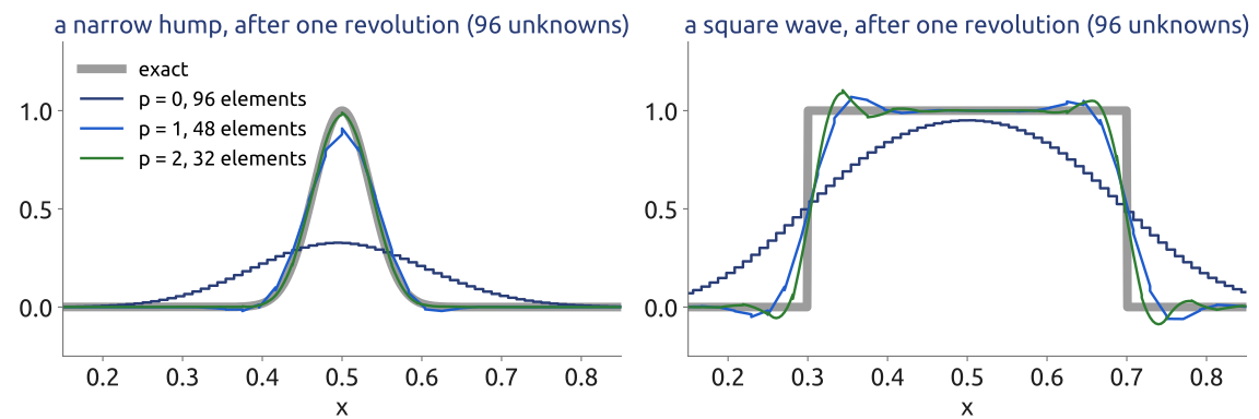
The scheme of the previous sections fits in a few lines of code. With the same number of unknowns, 96, DG with \(p = 0\) (96 elements), \(p = 1\) (48) and \(p = 2\) (32) is run for one revolution on a narrow Gaussian hump and on a square wave (Figure 15), with the upwind flux and SSP-RK3. One step of DG with \(p = 0\) and forward Euler agrees with the donor-cell update to round-off.
16 What the computation showed
DG with \(p = 0\) smears everything: its numerical diffusion is large. \(p = 1\) and \(p = 2\) keep the hump almost exactly; the convergence slopes are 1, 2, 3 and 4 (Figure 13). Near the jumps of the square wave all higher-order schemes overshoot: by Godunov’s theorem a linear scheme that never creates new extrema is at most of first order. DG keeps the overshoots within a narrow band, since its errors stay local; limiters remove them, as in finite volumes, and hp-adaptivity uses a high degree where the solution is smooth and a low one near fronts. With the central flux instead of the upwind one, nothing damps the grid-scale noise (Cockburn 2003; Hesthaven and Warburton 2008).
17 From 1D to 2D: faces and normals
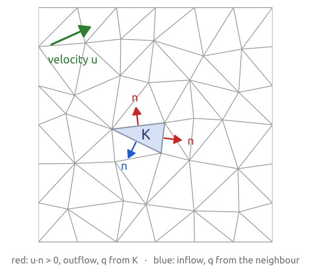
For a tracer \(q\) carried by a velocity \(\mathbf b\), \(\partial_t q + \nabla\cdot(\mathbf b\,q) = 0\), on a mesh of triangles or quadrilaterals, the same steps on each element \(K\) give \[ \int_K\partial_t q\,v\,dx - \int_K q\,\mathbf b\cdot\nabla v\,dx + \oint_{\partial K}\hat F\,v\,ds = 0, \qquad \hat F = (\mathbf b\cdot\mathbf n)\,q^{\text{up}}, \] with \(\mathbf n\) the outward unit normal of \(K\) and \(q^{\text{up}}\) the value on the side the flow comes from: from \(K\) where \(\mathbf b\cdot\mathbf n > 0\) (outflow), from the neighbour, or the boundary value, where \(\mathbf b\cdot\mathbf n < 0\) (Figure 16). Points become faces, and the formula is the same on triangles, squares or polygons (Hesthaven and Warburton 2008; Cockburn 2003).
18 Firedrake: the code is the weak form
Firedrake (Rathgeber et al. 2016) lets one write this weak form almost as it reads. In its language, UFL (also used by FEniCS), dx is an integral over the elements, dS over the interior faces, with the two sides '+' and '-', and ds over the boundary faces. With un = 0.5*(dot(u, n) + abs(dot(u, n))) \(= \max(\mathbf u\cdot\mathbf n, 0)\) on each side, the upwind flux summed over the two elements of an interior face is (phi('+') - phi('-'))*(un('+')*q('+') - un('-')*q('-'))*dS, with phi the test function. The volume term \(\int q\,\mathbf u\cdot\nabla\phi\,dx\) is q*dot(u, grad(phi))*dx (the integration by parts used \(\nabla\cdot\mathbf u = 0\), true for a solid-body rotation), and the boundary term takes the inflow value q_in where \(\mathbf u\cdot\mathbf n < 0\): phi*dot(u, n)*conditional(dot(u, n) < 0, q_in, q)*ds. Firedrake generates and compiles the element code and calls PETSc for the linear algebra; it runs in Google Colab through FEM on Colab.
19 DG advection in 2D, computed
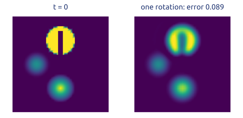
The solid-body rotation test of LeVeque (1996), after the Firedrake demo “DG advection equation with upwinding”: a cosine bell, a cone and a slotted cylinder rotate once about the centre of the unit square, with DG of degree 1 on \(40\times40\) squares and SSP-RK3 (Figure 17). After one rotation the relative \(L^2\) error is 0.089; the bell is kept, the tip of the cone and the edges of the cylinder are smoothed, with small over- and undershoots at the jumps. The total amount of \(q\) changes only through the boundary: in the interior DG conserves exactly, element by element.
20 Compatible elements (1/2): the C-grid, generalized
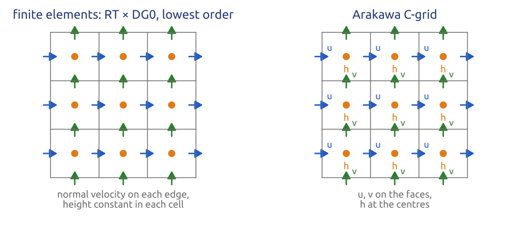
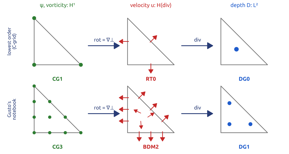
The shallow water equations need a space \(V^1\) for the velocity \(\mathbf u\) and a space \(V^2\) for the height \(\eta\) (the names of the de Rham complex below, as in Cotter and Thuburn (2014); Cotter and Shipton (2012) call them \(S\) and \(V\)). Compatible spaces satisfy \[ \nabla\cdot V^1 = V^2 : \] the divergence maps the velocity space onto the height space (Cotter and Shipton 2012). Examples are the Raviart–Thomas and Brezzi–Douglas–Marini spaces for \(V^1\) (vector fields whose normal component is continuous across edges, the \(H(\mathrm{div})\) spaces) with discontinuous polynomials for \(V^2\). The lowest pair on squares, lowest-order Raviart–Thomas (RT0) × DG0, has one normal velocity per edge and one height per cell: exactly the unknowns of the Arakawa C-grid (Figure 18); BDM1 × DG0 is the simplest pair on triangles. Firedrake calls RT0 “RT” (“RTCF” on squares) of degree 1, counting the degree of the full polynomial space.
21 Compatible elements (2/2): energy and balance
Multiply the linear rotating shallow water equations, \(\partial_t\mathbf u + f\,\mathbf u^\perp + g\nabla\eta = 0\) and \(\partial_t\eta + H\nabla\cdot\mathbf u = 0\), with \(\mathbf u^\perp = \mathbf k\times\mathbf u\) and the mean depth \(H\), by test functions \(\mathbf w \in V^1\) and \(\phi \in V^2\), and integrate the pressure term by parts (periodic domain): \[ \int\mathbf w\cdot\partial_t\mathbf u + f\,\mathbf w\cdot\mathbf u^\perp - g\,(\nabla\cdot\mathbf w)\,\eta\,dx = 0, \qquad \int\phi\,\partial_t\eta + H\,\phi\,\nabla\cdot\mathbf u\,dx = 0 . \] Compatible spaces keep the good properties of the C grid:
- Energy. Taking \(\mathbf w = H\mathbf u\) and \(\phi = g\eta\), allowed since they lie in \(V^1\) and \(V^2\), and adding gives \(\frac{d}{dt}\frac12\int H|\mathbf u|^2 + g\eta^2\,dx = -fH\int\mathbf u\cdot\mathbf u^\perp dx = 0\): the discrete energy is conserved exactly, and with the implicit midpoint rule in time also by the fully discrete scheme.
- Geostrophic balance. On triangles the spaces CG2 → BDM1 → DG0 form a discrete de Rham complex: for \(\psi\) in CG2, \(\nabla^\perp\psi\) lies in BDM1 and is divergence-free, and the divergence of BDM1 is DG0. Take \(\mathbf u = \nabla^\perp\psi\) and \(\eta = P_{V^2}(f\psi/g)\). Since \(\mathbf u^\perp = -\nabla\psi\), for every \(\mathbf w\), \(\int f\mathbf w\cdot\mathbf u^\perp - g(\nabla\cdot\mathbf w)\eta\,dx = \int(\nabla\cdot\mathbf w)(f\psi - g\eta)\,dx = 0\), because \(\nabla\cdot\mathbf w \in V^2\): every such balanced state is an exact steady state of the discrete equations (Cotter and Shipton 2012).
- No spurious pressure modes (heights with a zero discrete gradient), unlike equal-order pairs. The ratio of the numbers of unknowns also matters: two velocity unknowns per height unknown, as on the square C-grid, avoids spurious wave branches (RT\(_{k+1}\) × DQ\(_k\) on quadrilaterals, BDFM1 × DG1 on triangles); BDM1 × DG0 has three, like the hexagonal C-grid, and supports spurious Rossby-wave branches (Cotter and Shipton 2012).
22 Shallow water with Firedrake, computed
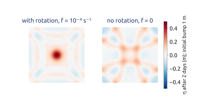
The linear rotating shallow water equations with BDM1 × DG0 on a doubly periodic square of 2000 km (48 × 48 × 2 triangles) and the implicit midpoint rule, \(H = 10\) m and \(f = 10^{-4}\) s\(^{-1}\), so \(\sqrt{gH} \approx 9.9\) m/s and \(L_d = \sqrt{gH}/f \approx 99\) km. A Gaussian bump of water 1 m high and 150 km in radius, released from rest, adjusts: without rotation it collapses completely and leaves as gravity waves; with rotation part of it stays as a balanced anticyclone (Figure 19). A balanced state built from a streamfunction, as in the previous section, stays steady.
23 What the Firedrake computations showed
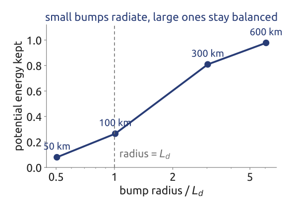
The DG advection run conserves \(q\) in the interior exactly, with an error of 0.089 after one rotation and small overshoots at jumps. The shallow water run conserves the energy to \(2\times10^{-15}\) in two days, and the balanced state changes by \(10^{-14}\): round-off. What stays after the adjustment depends on the size of the bump against the deformation radius: about 8% of the potential energy for a radius \(L_d/2\), 81% for \(3L_d\) (Figure 20); a 50 km bump is also poorly resolved, with cells of about 40 km (Cotter and Shipton 2012; Vallis 2017, sec. 3.9).
24 Gusto: a dynamical core from these pieces
Gusto is a Python library, built on Firedrake, for compatible finite element dynamical cores, developed at Imperial College London and the Met Office with the University of Exeter, a test bed for the compatible methods that underpin LFRic, the Met Office’s next model (Bendall et al. 2020; Shipton et al. 2018). It solves the shallow water, Boussinesq, compressible and moist Euler equations and runs the standard test cases. A run needs a mesh of the sphere, a family of compatible spaces, the equations in weak form, a time stepper and diagnostics (Figure 21). Which spaces, and why those, is the subject of the next section.

25 Compatible spaces: the de Rham complex
On a surface such as the sphere the compatible spaces form a discrete de Rham complex, \(H^1 \xrightarrow{\nabla^\perp} H(\mathrm{div}) \xrightarrow{\nabla\cdot} L^2\), with \(\nabla\cdot\nabla^\perp = 0\); the discrete spaces are \(V^0 \subset H^1\), \(V^1 \subset H(\mathrm{div})\) and \(V^2 \subset L^2\) (Cotter and Thuburn 2014; Cotter and Shipton 2012; Natale et al. 2016) (Figure 22). The streamfunction and the vorticity live in the continuous space \(H^1\), the velocity in \(H(\mathrm{div})\) (only its normal component is continuous across the edges), the depth in the discontinuous space \(L^2\). The discrete spaces keep the two identities of the continuous ones: the divergence maps the velocity space onto the depth space, and the rotated gradient of a discrete streamfunction has exactly zero divergence. At the lowest order on triangles (CG1, RT0, DG0) the unknowns are those of a C-grid on triangles; the Gusto runs below use degree 1 (CG3, BDM2, DG1). The vorticity is diagnosed in \(H^1\) from \(\int\gamma\,\zeta\,dA = -\int\nabla^\perp\gamma\cdot\mathbf u\,dA\) for every test function \(\gamma\).
26 Weak form in Gusto (1/2): the fast waves
Gusto writes the shallow water equations in the vector-invariant form \[ \partial_t\mathbf u + (\zeta + f)\,\mathbf u^\perp + \nabla\!\left(g(D + b) + \tfrac12|\mathbf u|^2\right) = 0, \qquad \partial_t D + \nabla\cdot(D\mathbf u) = 0 , \] with the relative vorticity \(\zeta\), the fluid depth \(D\) and the height of the orography \(b\). The fast terms, which carry the gravity waves and the rotation, linearized about rest, \(D = H + \eta\), are those of the linear system of compatible elements, now on the sphere, where integrating the pressure term by parts leaves no boundary term: \(\int\mathbf w\cdot\partial_t\mathbf u + f\,\mathbf w\cdot\mathbf u^\perp - g(\nabla\cdot\mathbf w)\eta\,dA = 0\) and \(\int\phi\,\partial_t\eta + H\phi\nabla\cdot\mathbf u\,dA = 0\). Only the divergence of the velocity appears: the velocity needs to be in \(H(\mathrm{div})\) only, and the depth needs no derivative at all (Cotter and Shipton 2012; Shipton et al. 2018). The full nonlinear terms enter the residual; this linear part is what the implicit solver inverts.
27 Weak form in Gusto (2/2): DG transport
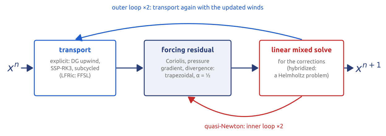
The slow terms, transport by the wind, are discretized as DG: on each triangle \(K\), \(\int_K\phi\,\partial_t D - \int_K\nabla\phi\cdot\mathbf u\,D + \oint_{\partial K}\phi\,(\mathbf u\cdot\mathbf n)\,\tilde D = 0\) with the upwind value \(\tilde D\) on each edge, which conserves the mass exactly. In Gusto’s current shallow-water set-up the vorticity and kinetic-energy terms of the velocity equation are integrated by parts and upwinded at the edges in the same spirit; Shipton et al. (2018), who introduced these spaces on the sphere, instead transported a potential vorticity held in the continuous space with a stabilized (Taylor–Galerkin) scheme and derived the vorticity term from it. Transport of the depth is explicit, SSP-RK3 with two substeps per step (the velocity’s transport terms use the trapezium rule), and so is limited only by the wind: about 40 m/s against gravity waves of 240 m/s, a transport Courant number six times smaller (Shipton et al. 2018; Bendall et al. 2020). LFRic has since replaced its transport by a conservative flux-form semi-Lagrangian scheme, stable at large Courant numbers (Bendall and Kent 2025).
28 One time step: semi-implicit quasi-Newton
The fast terms are implicit, with the trapezoidal rule, which gives a nonlinear system; Gusto solves it with two quasi-Newton iterations, each one a linear solve for the corrections with the equations linearized about a fixed state at rest (depth \(H\), rotation \(f\)): the same matrix every step, a Helmholtz problem on the mesh, which can be hybridized: Lagrange multipliers on the edges leave a smaller, sparse problem for the multipliers alone, with the spectral properties of a Helmholtz operator (Shipton et al. 2018, sec. 2.3.1). Transport and the iterations are repeated twice, an outer loop with the updated winds (Figure 23) (Shipton et al. 2018, sec. 2.3; Bendall et al. 2020, sec. 3.2; Melvin et al. 2019). The gravity waves no longer limit the time step: Gusto runs case 2 of the next sections stably with steps of 4 hours, a gravity-wave Courant number of 5.5, and LFRic runs at up to 10 (20 km, 10 min). This semi-implicit structure is that of most global models: the Met Office’s ENDGame and the IFS have it with semi-Lagrangian transport (Wood et al. 2014).
29 LFRic: GungHo in operation
The Met Office’s new atmosphere model, named after Lewis Fry Richardson, replaces the Unified Model. Its GungHo dynamical core keeps the structure of its predecessor ENDGame and changes its discretization: the latitude–longitude grid becomes an equiangular cubed sphere (no pole); finite differences on a C-grid become lowest-order compatible finite elements, the finite element equivalent of the C-grid, and of the Charney–Phillips staggering in the vertical; the equations stay the non-hydrostatic, deep-atmosphere compressible Euler equations, the time step stays semi-implicit, and semi-Lagrangian transport becomes a conservative flux-form semi-Lagrangian scheme (Melvin et al. 2019, 2024; Bendall and Kent 2025). The GungHo project began in 2011; compatible finite elements were chosen in 2013 and the cubed sphere in 2015; the model ran with full physics in 2022, and its first parallel suite is planned for 2027, to become the operational model in 2028 (T. Bendall, PDEs on the Sphere, São Paulo, 2025). The reasons: no pole and better scalability, local conservation, portability to new computers through code generation (PSyclone, as in Firedrake), and modern data assimilation.
30 Shallow water on the sphere with Gusto, computed
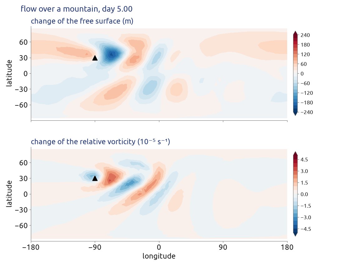
Two of the standard tests of Williamson et al. (1992) on Gusto’s icosahedral mesh with 8 cells per edge (1280 curved triangles; velocity in BDM2, depth in DG1: 9600 velocity and 3840 depth unknowns) and time steps of one hour. Case 2 is a zonal flow in exact geostrophic balance: it must stay steady. Case 5 puts a conical mountain 2000 m high, centred at 30°N, 90°W, in a zonal flow of 20 m/s; the animation shows five days of it (Figure 24). What happens follows from the conservation of the shallow-water potential vorticity \(Q = (\zeta + f)/D\) by each fluid column. Over the mountain the column is squashed, \(D\) falls, and so does \(\zeta + f\): the relative vorticity becomes negative there, an anticyclonic turning (in the run, \(-1.5\times10^{-6}\) s\(^{-1}\) on average over the mountain after five days). Downstream, a column pushed north finds a larger \(f\), its \(\zeta\) decreases and it turns back south, and the other way round: the increase of \(f\) with latitude, \(\beta = 2\Omega\cos\varphi/a\), is the restoring force of a Rossby wave. The wave that stands still in the flow has \(U = \beta/K^2\), a wavelength \(2\pi\sqrt{U/\beta}\), about 5900 km (some 60° of longitude) at 30°N with \(U \approx 17\) m/s; its energy can only travel east, so the wave train grows downstream (Vallis 2017, sec. 6.4 and §16.7). The notebook also writes the weak form as Gusto builds it, with the vorticity term integrated by parts and upwinded on the edges (Gusto’s current set-up, simpler than the potential-vorticity scheme of Shipton et al. (2018)), and the depth transported by upwind DG.
31 What the Gusto computation showed
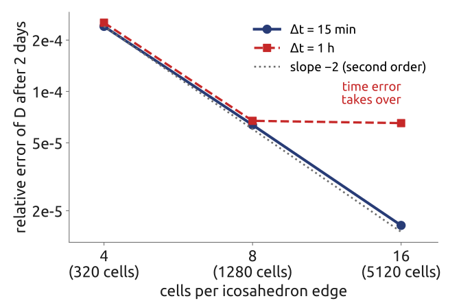
After two days the depth of case 2 differs from the exact solution by a relative \(6.7\times10^{-5}\), at a gravity-wave Courant number of 1.4, where an explicit scheme would be unstable. The error is of second order in space: with steps of 15 minutes it is \(2.4\times10^{-4}\), \(6.4\times10^{-5}\) and \(1.6\times10^{-5}\) for 4, 8 and 16 cells per edge, four times smaller each time the triangles are halved. With steps of one hour, however, the error at 16 cells per edge stays at \(6.5\times10^{-5}\): the time error has become larger than the space error, and refining the mesh alone no longer helps (Figure 25): space and time must be refined together (Williamson et al. 1992; Shipton et al. 2018). In case 5 the conservation of \(Q\) gives the stationary Rossby wave train; without rotation (\(f = 0\), no \(\beta\)) there is none, and the surface changes by a few tens of metres only. The pair of spaces matters: the triangular C-grid (velocity in RT0, depth in DG0; Firedrake’s RT1) has about 60 times the error of BDM2 × DG1 in case 2, and its ratio of 3 velocity to 2 depth unknowns gives the linear waves a spurious branch of inertia–gravity modes, which shows as checkerboard patterns in the divergence when the deformation radius is small (Cotter and Shipton 2012; Cotter and Thuburn 2014). Here \(L_d = \sqrt{gH}/f \approx 2400\) km (with \(f = 10^{-4}\) s\(^{-1}\)), many cells wide, and the 5-day run shows no checkerboard. A 2:1 pair (velocity in BDFM1, depth in DG1; Firedrake’s BDFM2) has no spurious branch, and here the accuracy of BDM2 × DG1.
32 Finite elements in weather and climate models
- LFRic (Met Office, UK): the GungHo core, lowest-order compatible finite elements for the dynamics and finite volumes for transport, on a cubed-sphere mesh; the operational model from 2028 (Adams et al. 2019; Melvin et al. 2019). LFRic does not use Firedrake: it is written in Fortran 2003 with a separation of concerns between the science code and the parallel code (the PSyKAl layers: algorithm, parallel system, kernels), and the code generator PSyclone (STFC Hartree Centre) writes the parallel layer from metadata in the kernels (Adams et al. 2019). Gusto, in Python on Firedrake, is a test bed for its compatible methods.
- Spectral elements: continuous Galerkin with high-order polynomials on quadrilaterals, with the nodes at the Gauss–Lobatto–Legendre points so that the mass matrix is diagonal. They are used in KIM, the Korean Integrated Model of KIAPS for global weather forecasting, on the cubed sphere (Choi and Hong 2016; Hong et al. 2018); in CAM-SE/HOMME (NCAR, and the US Department of Energy’s E3SM) on the cubed sphere (Dennis et al. 2012; Taylor and Fournier 2010); in NUMA, the core of NEPTUNE, the US Navy’s model (closed code), on any quadrilateral mesh (Kelly and Giraldo 2012); and in the horizontal of the CliMA atmosphere model (ClimaAtmos), on the cubed sphere, with finite differences in the vertical (Yatunin et al. 2025).
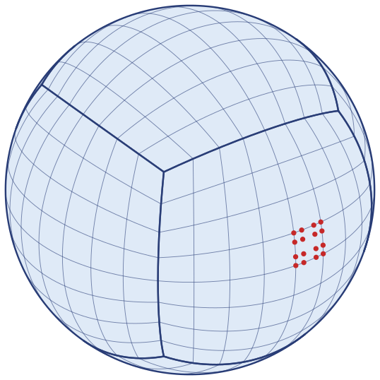
These models use the cubed-sphere mesh of Figure 26: six patches of quadrilaterals, with no pole problem. Element methods scale because each element talks only to its neighbours.
33 Finite elements and DG in ocean models
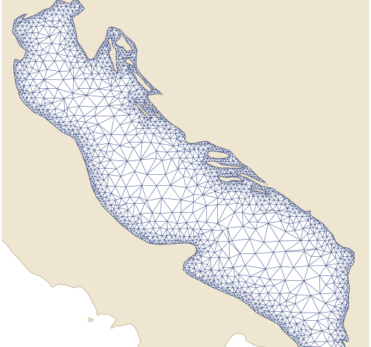
In the ocean, finite elements are rare. Global ocean and climate models are finite-difference or finite-volume codes on structured grids: of the eleven models of the Ocean Model Intercomparison Project (OMIP-2), ten use structured B or C grids (NEMO, MOM, POP, HYCOM, MPIOM and others), and the exception, FESOM 1.4, was the only one on an unstructured mesh (Tsujino et al. 2020; Fox-Kemper et al. 2019). Finite elements live on the coast, where an unstructured mesh draws the coast, the islands and the estuaries as they are, with small cells only where they are needed (Figure 27).
- Continuous Galerkin or hybrid finite element and finite volume models: ADCIRC, for storm surge and tides on meshes from the ocean basin to the channels of a delta (Westerink et al. 2008), runs NOAA’s operational global tide and surge forecasts (STOFS-2D-Global); SCHISM (and its predecessor SELFE), from creeks to the open ocean (Zhang et al. 2016), runs NOAA’s operational Atlantic forecasts (STOFS-3D-Atlantic; NWS notice SCN26-51, 2026); SHYFEM (CNR-ISMAR) forecasts tides and surge in the Adriatic and the Venice lagoon (Umgiesser et al. 2004; Ferrarin et al. 2013; Cirano et al. 2025); FESOM 1.4, the first global ocean general circulation model on unstructured meshes developed for climate research, AWI’s ocean in CMIP6 (Wang et al. 2014). Continuous elements suit elliptic problems, but advection needs stabilization and the coupled global system is less efficient in parallel than finite volumes (Kärnä et al. 2018). FESOM2 replaced its finite elements with finite volumes and became at least three times faster while keeping the fidelity of its simulations (Danilov et al. 2017).
- Adaptive finite elements: Fluidity (the Imperial College Ocean Model) changes its unstructured tetrahedral mesh in time to follow the evolving solution, with long thin elements aligned with boundary layers (Piggott et al. 2008).
- Discontinuous Galerkin: local and fully conservative like finite volumes, well suited for advection, and of higher order, but so far in research codes. SLIM (Second-generation Louvain-la-Neuve Ice-ocean Model) uses DG on unstructured prismatic meshes (Blaise et al. 2010; Delandmeter et al. 2018); Thetis, a DG coastal ocean model for the three-dimensional hydrostatic equations, is written on Firedrake (Kärnä et al. 2018).
34 Research: DG on Voronoi meshes
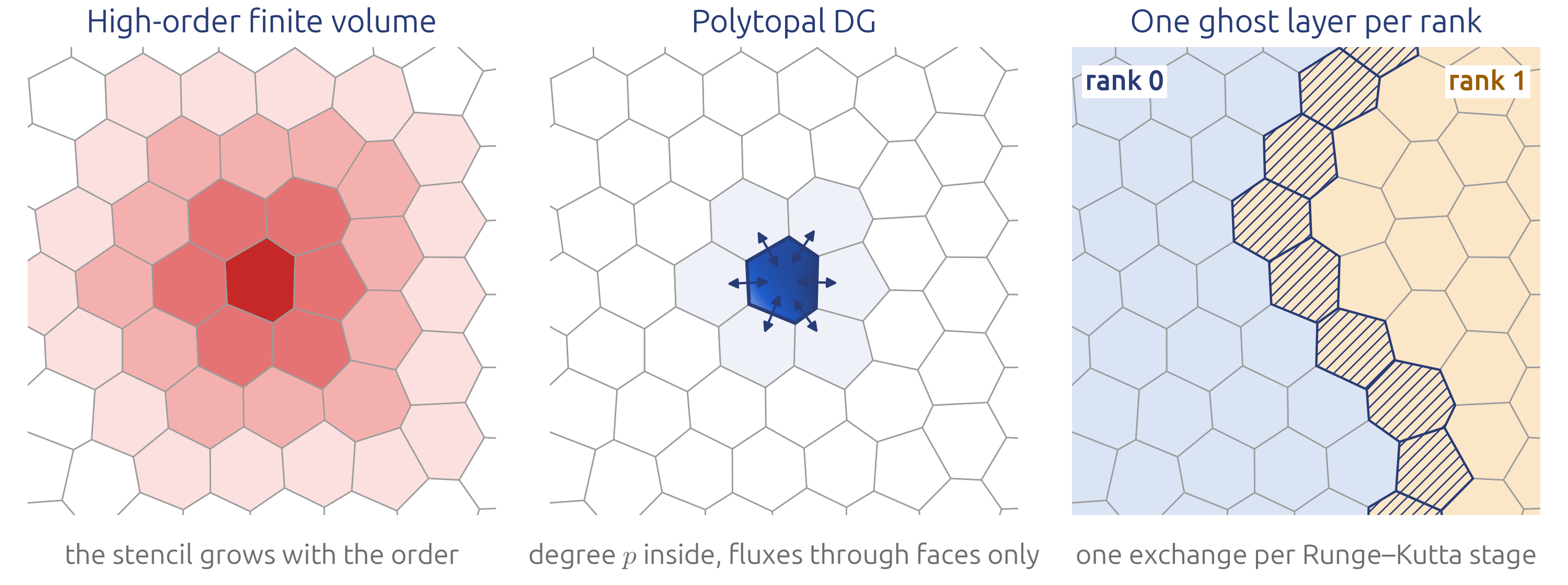
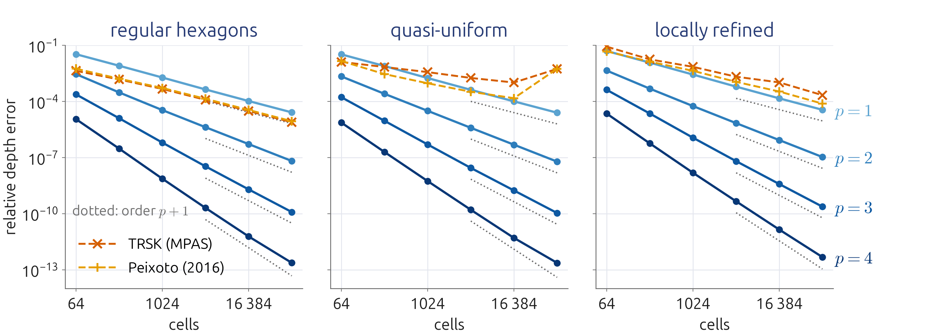
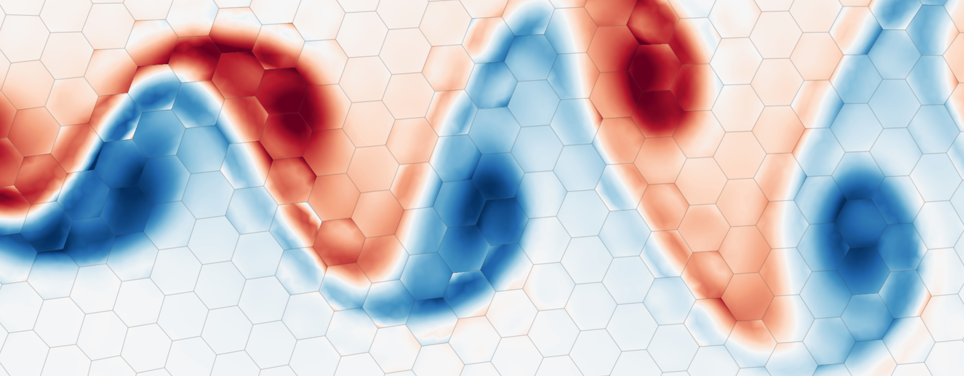
Polytopal DG (PolyDG, with MOX) for the rotating shallow water equations on Voronoi meshes, as in MPAS, aims at high order with the locality of finite volumes on the meshes of operational models (Figure 28). It converges with order \(p + 1\) on every mesh, also on irregular and locally refined ones, where the finite volumes of MPAS (the TRSK scheme) lose accuracy (Figure 29), and local refinement leaves no visible imprint on an unstable jet (Figure 30) (Marras et al. 2016).
35 A vertical slice with Gusto
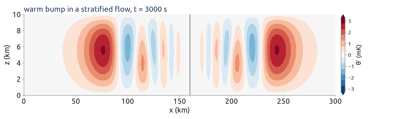
An extra, not done in class. The same compatible spaces on an extruded mesh of a vertical slice (150 columns of 2 km, 10 layers of 1 km) solve the compressible Euler equations, sound waves included. In each cell the horizontal velocity sits on the sides, the vertical velocity on the top and bottom, the density inside: the C-grid in the \(x\)–\(z\) plane; the potential temperature shares the points of the vertical velocity, the Charney–Phillips staggering (Bendall et al. 2020). The test of Skamarock and Klemp (1994) puts a warm bump of 0.01 K, 5 km wide, in a stratified channel (\(N = 0.01\) s\(^{-1}\)) with a wind of 20 m/s: the bump, carried by the wind, splits into internal gravity waves, the long ones ahead, with \(\omega = N\cos\alpha\) (Figure 31). After 3000 s the maximum of \(\theta'\) is 2.80 mK against 2.73 mK from linear Boussinesq theory, and the semi-implicit step is stable at a sound-wave Courant number of 4 (steps of 12 s on layers of 1 km).
36 Key points
- Weak form: multiply by a test function, integrate, by parts: fewer derivatives on the unknown.
- Galerkin: trial and test functions from the same space; stiffness and mass matrices (hats: the finite-difference Laplacian).
- DG = a polynomial in each element + numerical fluxes at the faces; upwind; block-diagonal mass matrix.
- Order \(p + 1\); time step \(\sim 1/(2p+1)\); DG with \(p = 0\) = upwind finite volumes.
- Compatible elements (\(\nabla\cdot V^1 = V^2\)): the C-grid on any mesh; energy and geostrophic balance kept; Gusto and LFRic build dynamical cores from them.
- Firedrake: the weak form as code.
Finite elements: local, high order, on any mesh, and still conservative.
Further reading
Durran (2010), §6.5–6.6 (finite elements and DG for geophysical problems); Hesthaven and Warburton (2008), a practical book on nodal DG with codes; Cockburn (2003), a short introduction to DG; Cotter and Shipton (2012) for compatible finite elements in weather prediction; Marras et al. (2016) for a review of element-based methods in numerical weather prediction.