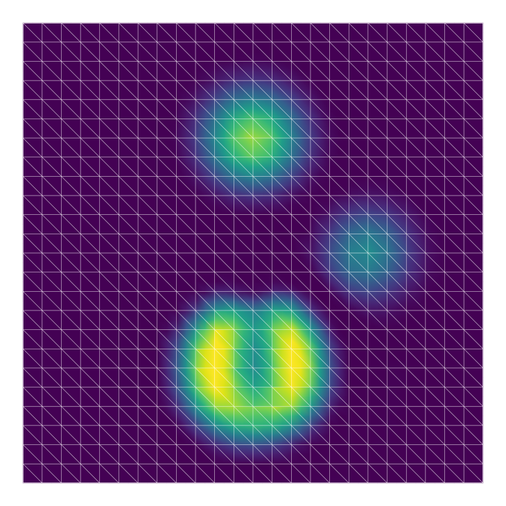
December 2026 · Politecnico di Milano

Finite elements: from Galerkin to discontinuous Galerkin

Atmosphere and Ocean Dynamics — Lecture 8

Prof. Dr. Pedro da Silva Peixoto

Applied Mathematics
Instituto de Matemática e Estatística
Universidade de São Paulo

Visiting Professor at MOX Lab
Politecnico di Milano

Warm-up

1. The spectral derivative of \(e^{ikx}\) on a grid of \(M\) points: what is its error for \(|k| < M/2\)?
2. On \(M\) grid points, which wave looks like \(k = 1\)? How many points per shortest wave avoid aliasing in \(u^2\)?
3. \(\nabla^2 Y_n^m = \;\)? Why does this make the Poisson and Helmholtz problems cheap?
4. Double the resolution of a spectral model: how much more work for one Legendre transform? Why is communication a problem on large computers?

Lecture 7, from memory: answer on paper first, 3 minutes (its carry-forward list).

Answers: 1. none: exact (k_eff = k). 2. k = 1 ± M, …; three (M ≥ 3N + 1, the 2/3 rule; N the truncation). 3. −n(n+1)Y/a²: a division per coefficient. 4. ×8 (T³); every coefficient needs every grid point: global transpositions every step. Today: local methods.

Where we are and where we are going

Previous knowledge

• Spectral derivatives are exact for every resolved wave, \(|k| < M/2\) on \(M\) points
• Aliasing: on \(M\) points \(k = 1\) looks like \(k = 1 \pm M\); products \(u^2\) need three points per shortest wave (\(M \ge 3N + 1\) for truncation \(N\), the 2/3 rule)
• \(\nabla^2 Y_n^m = -n(n+1)\,Y_n^m/a^2\): a Poisson or Helmholtz problem is one division per coefficient
• Double the resolution: Legendre transforms cost 8 times more; every coefficient needs every grid point: global communication every step
• Integration by parts, Gauss’s theorem; finite volumes: cell averages, face fluxes, donor cell; the C-grid

Where we are going

1. Why local? The weak form, Galerkin’s hats
2. Discontinuous Galerkin: fluxes, \(p = 0\)
3. High order and the time step; notebook
4. DG in 2D with Firedrake
5. Compatible elements for shallow water
6. Gusto and LFRic
7. Finite elements in weather and climate models

Local polynomials glued by fluxes: finite volumes that reach high order on any mesh

(Durran 2010, secs. 6.5–6.6; Cotter and Shipton 2012)

Two minutes. Left: what we take as known (lectures 3, 6, 7; the warm-up checked it). Right: the road of the day; each item links to its first slide.

Why local?

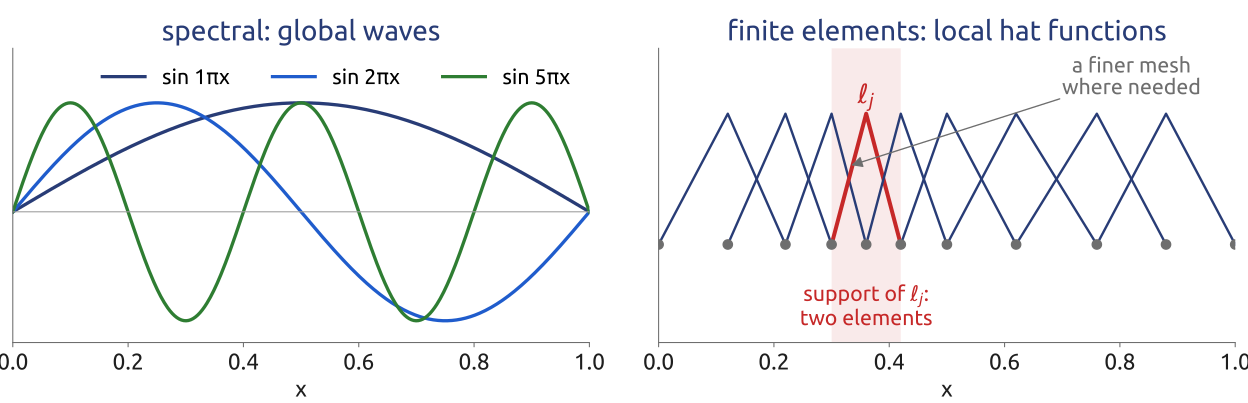
• Spectral: each coefficient talks to the whole globe: global communication

• Finite elements: local functions on any mesh, refined where needed; high order inside each element

Finite elements: local basis functions on any mesh

(Durran 2010, sec. 6.5; Marras et al. 2016)

Spectral transforms: lecture 7. Same idea as spectral (a sum of basis functions), but each basis function lives on a few elements.

Weak form (1/4): multiply and integrate

Model problem: the 1D Poisson problem

\[-u'' = f \text{ on } (0, 1), \qquad u(0) = u(1) = 0\]

\(u\): the unknown; \(f\): a given source; a prime: \(d/dx\)

Multiply by a test function \(v\), with \(v(0) = v(1) = 0\), and integrate:

\[\int_0^1 \big(-u'' - f\big)\,{\color{#1f5ccc} v}\;dx = 0 \quad\text{for every } v\]

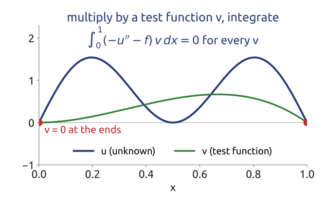
Multiply by a test function and integrate: one equation for every test function

(Durran 2010, sec. 6.5; Hesthaven and Warburton 2008)

“For every v” recovers the equation: if the integral vanishes for all v, the bracket is zero.

Weak form (2/4): integrate by parts

\[-\int_0^1 u''v\,dx = \int_0^1 u'v'\,dx - \big[u'v\big]_0^1\]

The boundary term vanishes (\(v = 0\) at the ends):

\[{\color{#1f5ccc}\int_0^1 u'\,v'\,dx} = \int_0^1 f\,v\,dx \quad\text{for every } v\]

• Choices of test functions?
• Only first derivatives: a function with kinks is allowed

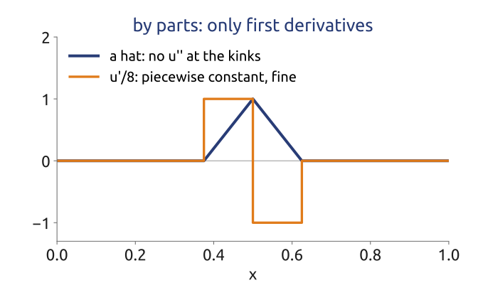
Integration by parts moves a derivative onto the test function: kinks are allowed

(Durran 2010, sec. 6.5)

The weak form: find u in H¹₀ such that a(u, v) = (f, v) for all v in H¹₀. Lax–Milgram (notes, aside).

Galerkin (3/4): a finite set of hats

Take \(u_h\) and \(v\) from the same finite space, the hat functions \(\ell_j\) (linear Lagrange functions):

\[u_h = \sum_j U_j\,\ell_j, \qquad v = \ell_i\] \[\sum_j \underbrace{\int\ell_i'\ell_j'\,dx}_{S_{ij}}\,U_j = \underbrace{\int f\,\ell_i\,dx}_{F_i}\]

\(\ell_j\): 1 at node \(x_j\), 0 at the others; \(U_j\): nodal values; \(S\): stiffness matrix

• One equation per unknown: \(SU = F\)
• \(S_{ij} \ne 0\) only if \(\ell_i\), \(\ell_j\) overlap: a sparse matrix

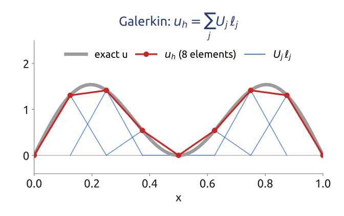
Galerkin: one equation per basis function, a sparse linear system

(Durran 2010, sec. 6.5.1)

Galerkin: trial and test functions from the same space. Here u_h equals u at the nodes (a 1D property).

Galerkin (4/4): the matrices

On a uniform mesh of size \(h\), only neighbours overlap:

\[\begin{aligned} S &= \frac{1}{h}\,\mathrm{tridiag}(-1,\,2,\,-1) && \text{(stiffness)}\\ M &= \frac{h}{6}\,\mathrm{tridiag}(1,\,4,\,1) && \text{(mass)} \end{aligned}\]

• Row \(j\) of \(SU = F\): \(\dfrac{-U_{j-1} + 2U_j - U_{j+1}}{h^2} \approx f_j\), the centred difference
• \(M_{ij} = \int\ell_i\ell_j\,dx\) appears with \(\partial_t u\)

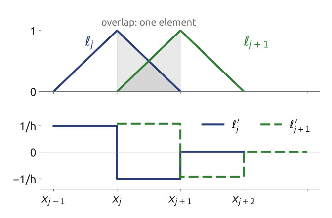
Linear elements on a uniform mesh: the stiffness matrix is the finite-difference Laplacian

(Durran 2010, sec. 6.5.1)

Ask first: what is ∫ℓ_j’ ℓ_{j+1}’ dx? (−1/h.) The difference from FD: any mesh, any degree, and a proof of convergence (Céa’s lemma, notes).

Continuous Galerkin for advection

From now on a problem in time, transport:

\[u_t + c\,u_x = 0\]

\(u\): the transported field; \(c\): constant advection speed; periodic domain

Hats (P1): \(M\dot U = -c\,\big[\textstyle\int\ell_i\ell_j'\,dx\big]\,U\); row \(j\):

\[\frac{\dot U_{j-1} + 4\dot U_j + \dot U_{j+1}}{6} = -c\,\frac{U_{j+1} - U_{j-1}}{2h}\]

\(U_j\): nodal values; \(\dot U_j = dU_j/dt\); \(k\): wavenumber; \(\omega\): numerical frequency

• Phase error of 4th order: \(\omega = \dfrac{3c\sin kh}{h(2 + \cos kh)}\)

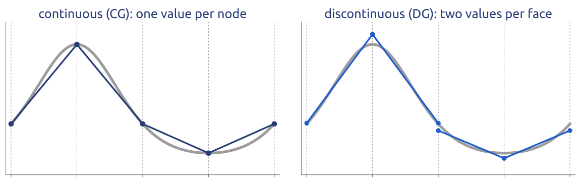
Continuous: one value per node. Discontinuous: two values per face.

 

But: \(M^{-1}\) couples all unknowns, a global solve every step; and nothing damps the noise

Let the solution jump between elements: discontinuous Galerkin

(Durran 2010, sec. 6.5.1; Hesthaven and Warburton 2008)

∫ ℓ_i ℓ_j’ dx = (−1/2, 0, 1/2) on a uniform mesh. Inverting M: a tridiagonal (cyclic) solve per step; in 2D/3D a sparse global solve. “Mass lumping” (diagonal M) loses the accuracy.

DG (1/4): a polynomial in each element

Broken space: on each element \(K_j\), a polynomial of degree \(p\); no continuity between elements:

\[V_h = \{\,v :\; v|_{K_j} \in \mathbb P_p \text{ for every } K_j\,\}\]

\(\mathbb P_p\): polynomials of degree \(\le p\); \(K_j\): the elements

• \(p + 1\) unknowns per element

But: what happens at the faces, where \(u_h\) jumps?

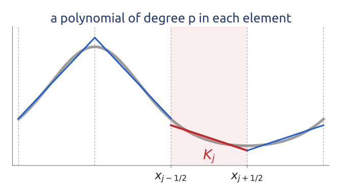
DG: a polynomial in each element, free to jump at the faces

(Cockburn 2003; Hesthaven and Warburton 2008)

Reed & Hill (1973) introduced DG for neutron transport; Cockburn and Shu developed it for conservation laws (Cockburn 2003 for the history).

DG (2/4): integrate by parts in one element

Test with \(v\) that lives on \(K_j\) only; integrate over \(K_j\); move the derivative to \(v\):

\[\int_{K_j}\!\partial_t u_h\,v\,dx - \int_{K_j}\! c\,u_h\,\partial_x v\,dx + {\color{#1f5ccc}\Big[\hat F\,v\Big]_{x_{j-1/2}}^{x_{j+1/2}}} = 0\]

\(u_h\): the DG solution; \(\hat F\): the numerical flux at a face; \(x_{j\pm1/2}\): the faces of \(K_j\)

• The boundary terms are the fluxes through the two faces
• One element at a time: the equations are local

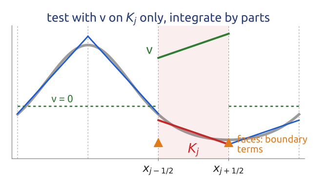
Integrated over one element, the equations meet the neighbours only at the faces

(Durran 2010, sec. 6.6; Hesthaven and Warburton 2008)

As in a finite volume: the integral form over the element, but with a polynomial instead of a constant, and for every test function of the element.

DG (3/4): the numerical flux

At a face, \(u_h\) has two values. Choose one flux, the same for both elements:

\[\hat F = c\,u^- \quad (c > 0): \textbf{upwind}\]

\(u^-\), \(u^+\): the values of \(u_h\) just left and right of the face

• Consistent: \(\hat F(u, u) = c\,u\)
• Conservative: what leaves \(K_j\) enters \(K_{j+1}\)
• Other choices: central \(c\,(u^- + u^+)/2\), Lax–Friedrichs, Riemann solvers

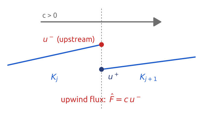
One flux per face, the same for both elements: consistent and conservative

(Cockburn 2003; LeVeque 2002)

Ask first: the wind blows from left to right. Which of the two values should cross the face? (u⁻, upstream.) The flux is the same idea as in finite volumes: an approximate Riemann problem at each face (lecture 6).

DG (4/4): local mass matrices

With \(u_h|_{K_j} = \sum_l U_{j,l}\,P_l\) and \(v = P_i\) (polynomials of degree \(\le p\), for instance Legendre):

\[M_K\,\frac{dU_j}{dt} = R\big(U_j,\; U_{j-1}\big)\]

\(U_j\): the coefficients of element \(j\); \(M_K\): its mass matrix; \(R\): volume and face terms

• \(M_K\): a small \((p+1)\times(p+1)\) block per element; Legendre polynomials make it diagonal
• Explicit Runge–Kutta, element by element, no global solve
• Each element needs only its neighbours: one layer of data exchange

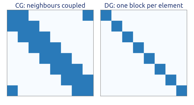
DG = a polynomial in each element + numerical fluxes at the faces

(Hesthaven and Warburton 2008; Cockburn 2003)

Left: CG mass matrix (periodic P1, couples neighbours); right: DG p = 1 (2 × 2 blocks).

p = 0: a finite-volume scheme

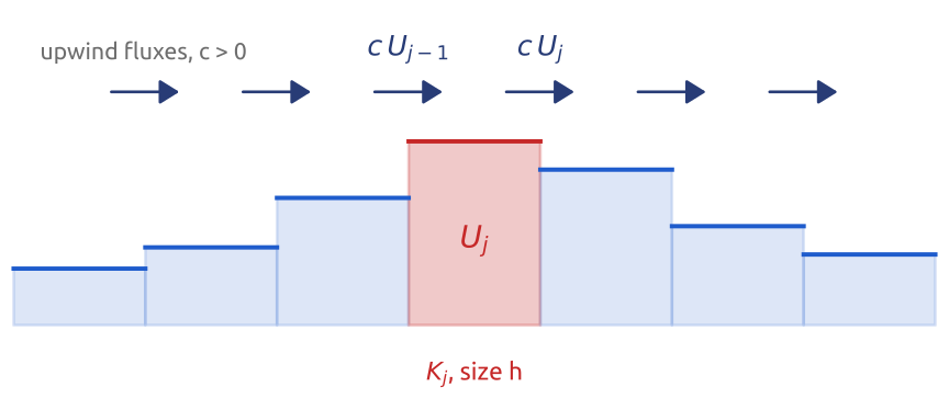
\(p = 0\): \(u_h = U_j\) on \(K_j\), \(v = 1\), \(\partial_x v = 0\):

\[h\,\frac{dU_j}{dt} = -\big(c\,U_j - c\,U_{j-1}\big)\]

\(U_j\): the mean of \(u\) on \(K_j\); \(h\): element size

The upwind (donor cell) finite-volume scheme

DG with p = 0 is the upwind finite-volume scheme: DG is finite volumes with polynomials inside

(Cockburn 2003; LeVeque 2002)

Ask first: with p = 0, which scheme of lecture 6 do you get? Every DG scheme contains a finite-volume balance: the test function v = 1 on K gives the conservation of the element average.

Higher order: a Legendre basis

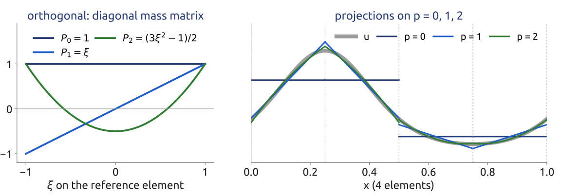
• Local coordinate \(\xi \in [-1, 1]\), \(x = x_j + h\xi/2\): \(\int_{K_j}P_iP_l\,dx = \dfrac{h}{2i+1}\,\delta_{il}\), a diagonal mass matrix

• Volume term: \(\int P_l\,P_i'\,d\xi\); faces: \(P_i(1) = 1\), \(P_i(-1) = (-1)^i\)

With orthogonal polynomials each element is a tiny spectral method

(Hesthaven and Warburton 2008; Durran 2010, sec. 6.6.1)

Modal basis (Legendre) here; nodal bases (Lagrange at Gauss–Lobatto points) are also common (Hesthaven & Warburton). Spectral elements: continuous, high-order, GLL nodes.

Order p + 1, and the time step

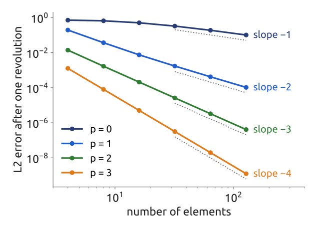
L2 error after one revolution of \(\sin 2\pi x\), periodic, \(c = 1\); upwind flux, SSP-RK3, Courant number \(0.1/(2p+1)\)

• Smooth solutions: error \(\sim h^{p+1}\)
• SSP-RK3 (Shu & Osher 1988): largest stable Courant number

\(p = 0\)	1.26
\(p = 1\)	0.41
\(p = 2\)	0.21
\(p = 3\)	0.13

Courant number \(c\Delta t/h\). For Runge–Kutta of order \(p+1\) the limit is \(1/(2p+1)\) (Cockburn 2003); for large \(p\) it falls like \(p^{-2}\) (Hesthaven & Warburton, §4.8)

Higher degree: much smaller errors for smooth fields, at a smaller time step

(Cockburn 2003, sec. 3.3; Hesthaven and Warburton 2008, sec. 5.7; Shu and Osher 1988; Gottlieb et al. 2001)

Ask first: if p = 2, what slope do you expect? (−3.) The Courant numbers are computed in notebook 08a from the eigenvalues of the scheme (Bloch analysis). SSP-RK3 is the third-order scheme of Shu & Osher (1988); the name “strong stability preserving” is from Gottlieb, Shu & Tadmor (2001). With RK of order p+1 the rule is 1/(2p+1) (Cockburn 2003), close to our numbers.

Dispersion and dissipation

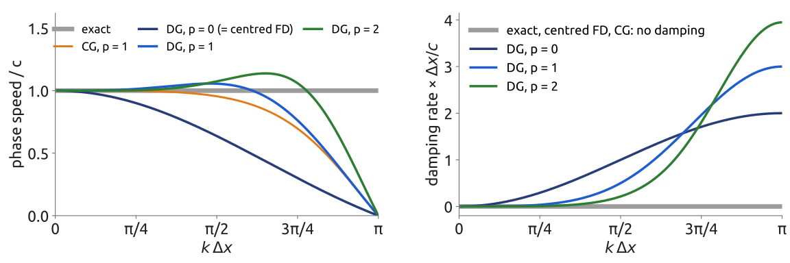
Semi-discrete (exact in time), a wave \(e^{ikx}\): \(du/dt = \lambda u\). Left: phase speed \(-\mathrm{Im}\,\lambda/k\) over \(c\); right: damping rate \(-\mathrm{Re}\,\lambda\). DG: \(\lambda\) of the physical mode of the element-to-element (Bloch) problem. \(\Delta x = h/(p+1)\): same number of unknowns

• DG \(p \ge 1\): resolved waves at almost the right speed

• Upwind flux: damps only the unresolved waves

DG moves the resolved waves at almost the right speed and damps only the unresolved ones

(Hesthaven and Warburton 2008; Durran 2010, sec. 6.6)

FD2 dispersion: lecture 5. Same number of unknowns: Δx = h/(p+1). DG p = 0 has the phase of the centred difference plus a strong damping (the numerical diffusion of the upwind scheme). Bloch analysis: the notes; notebook 08a, section 5, uses the same eigenvalues for the time step.

Notebook DG for advection in 1D

Notebook 08a (open in Colab · download): discontinuous Galerkin for advection in 1D, in a few lines of numpy.

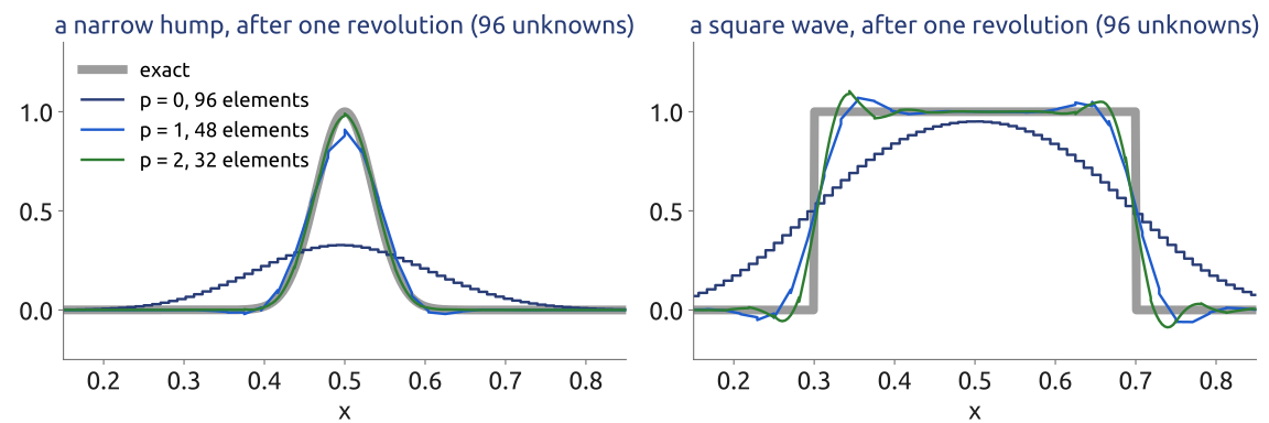
A hump and a square wave after one revolution, 96 unknowns: DG with p = 0, 1, 2

0. Galerkin with hat functions 🧩 0.1
1. The scheme: Legendre basis, upwind flux, SSP-RK3
2. \(p = 0\) is upwind finite volumes
3. Convergence for \(p = 0, \dots, 3\)
4. A hump and a square wave ❗ 4.1
5. The time step

Predict, run, explain: write down what you expect before each run

DG in a few lines: order \(p + 1\) where smooth, overshoots in a narrow band at jumps

(Hesthaven and Warburton 2008; Cockburn 2003)

In class, 25 min: sections 1 to 4; section 0 (optional) and section 5 at home. During the break, start the Firedrake install cell of 8b in Colab.

What the notebook showed

• \(p = 0\) and the upwind scheme agree to \(10^{-16}\)
• Slopes 1, 2, 3, 4; with 96 unknowns, \(p = 2\) keeps the hump, \(p = 0\) smears it
• Jumps: overshoots in a narrow band; DG with the upwind flux is a linear scheme
• Central flux: no damping, grid-scale noise

Godunov’s theorem (Godunov 1959). A linear scheme for the advection equation that never creates new extrema (monotonicity preserving) is at most first order accurate.

High order where the solution is smooth; the upwind flux keeps it clean

(Godunov 1959; Durran 2010, sec. 5.2; Cockburn 2003)

Godunov’s theorem and limiters: lecture 6. Linear: the coefficients do not depend on the solution. Limiters (as in FV) remove the overshoots at jumps; hp-adaptivity uses high p where smooth, low p near fronts.

From 1D to 2D: faces and normals

For \(\partial_t q + \nabla\cdot(\mathbf u\,q) = 0\) on each element \(K\) of a mesh:

\[\begin{gathered}\int_K \partial_t q\,v\,dx - \int_K q\,\mathbf u\cdot\nabla v\,dx + \oint_{\partial K}\hat F\,v\,ds = 0,\\ \hat F = (\mathbf u\cdot\mathbf n)\,q^{\text{up}}\end{gathered}\]

\(q\): tracer; \(\mathbf u\): velocity; \(\mathbf n\): outward normal of \(K\); \(q^{\text{up}}\): \(q\) on the upwind side

• Points become faces; the sign of \(\mathbf u\cdot\mathbf n\) picks the upwind side
• Triangles, squares, polygons: the same formula

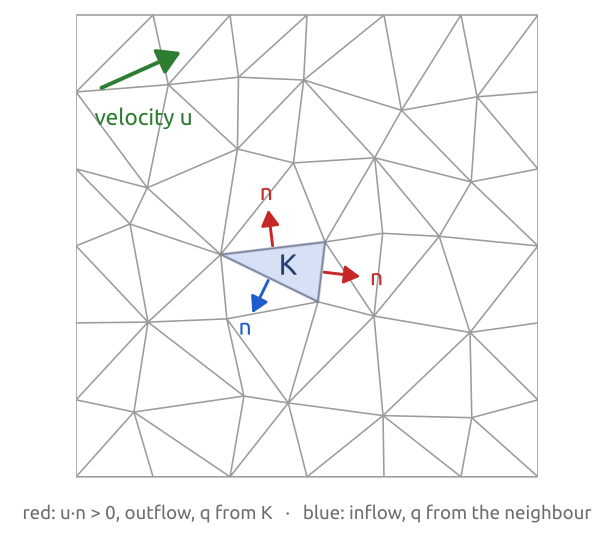
In 2D the same weak form: integrals over the element, fluxes through its faces

(Hesthaven and Warburton 2008; Cockburn 2003)

n: outward unit normal of K. Outflow faces (u·n > 0) use q from K; inflow faces from the neighbour (or the boundary value).

Firedrake: the code is the weak form

\[\int_K \phi\,\partial_t q\,dx = \int_K q\,\mathbf u\cdot\nabla\phi\,dx - \oint_{\partial K}\phi\,(\mathbf u\cdot\mathbf n)\,q^{\text{up}}\,ds\]

\(K\): one element, \(\partial K\): its boundary, \(\mathbf n\): outward normal; \(\phi\): test function; \(q^{\text{up}}\): the value of \(q\) on the upwind side

V   = FunctionSpace(mesh, "DQ", 1)      # broken polynomials
phi = TestFunction(V)
n   = FacetNormal(mesh)
un  = 0.5*(dot(u, n) + abs(dot(u, n)))  # max(u.n, 0)
a = phi*dq*dx                           # mass matrix
L = (q*dot(u, grad(phi))*dx             # volume term
     - (phi('+') - phi('-'))            # faces
       *(un('+')*q('+') - un('-')*q('-'))*dS
     - phi*dot(u, n)                    # boundary
       *conditional(dot(u, n) < 0, q_in, q)*ds)

• dx: elements; dS: interior faces, sides '+', '-'; ds: boundary
• Firedrake generates and compiles the code; PETSc solves
• Runs in Colab (FEM on Colab)

Write the weak form, Firedrake writes the code

(Rathgeber et al. 2016) · Demo: firedrakeproject.org: DG advection

UFL: the Unified Form Language (also used by FEniCS). q_in: the inflow value. dq: the increment dt·L(q) of an SSP-RK3 stage (one mass-matrix solve; one solver for the three stages). The jump of phi times the upwind flux sums the face terms of both elements.

Notebook DG advection in 2D with Firedrake

Notebook 08b (open in Colab · download): the weak form as code, DG advection on a 2D mesh with Firedrake.

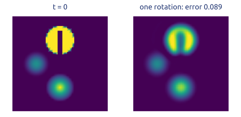
DQ1 on 40 × 40 squares: the initial shapes and one rotation

1. The problem: solid-body rotation of a bell, a cone and a slotted cylinder
2. The weak form in UFL, against the formula
3. The run: SSP-RK3, one rotation
4. Results: which shape survives best? ❗ 4.1 🧩 4.2

❗ 4.1: the polynomial degree. Predict, run, explain; the install cell first (a few minutes)

Write the weak form, run a 2D DG model

(Rathgeber et al. 2016; Hesthaven and Warburton 2008)

20 min in class if the install works, else at home. After LeVeque (1996) and the Firedrake demo. Exercise 4.1 (degree 0, 1, 2) is mandatory; 4.2 (triangles) optional.

Compatible elements (1/2): the C-grid, generalized

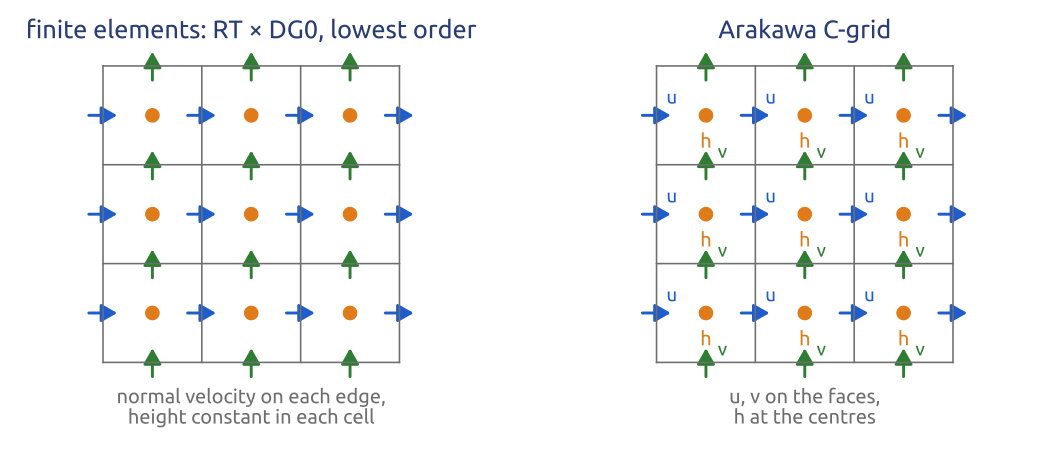
Shallow water: velocity \(\mathbf u \in V^1\), height \(\eta \in V^2\). Compatible:

\[\nabla\cdot V^1 = V^2\]

\(V^1\): velocity space, normal components continuous across edges; \(V^2\): height space, discontinuous

• Lowest-order Raviart–Thomas (RT0) × DG0 on squares: the C-grid
• Triangles: BDM1 × DG0, the simplest; higher orders; any mesh

Compatible finite elements: the C-grid on any mesh, at any order

(Cotter and Shipton 2012; Melvin et al. 2019)

Ask first: why did the C-grid beat the A-grid for gravity waves (lecture 6)? (The divergence and the height gradient live at the right places.) H(div): normal component continuous across edges. Names: the lowest-order Raviart–Thomas space is RT0 (as in Cotter & Shipton 2012); Firedrake calls it RT (“RTCF” on squares) of degree 1, as in the code of the notebooks.

Compatible elements (2/2): energy and balance

From \(\partial_t\mathbf u + f\mathbf u^\perp = -g\nabla\eta\), \(\partial_t\eta + H\nabla\cdot\mathbf u = 0\): test with \(\mathbf w \in V^1\), \(\phi \in V^2\); the gradient by parts:

\[\begin{aligned} \int \mathbf w\cdot\partial_t\mathbf u + f\,\mathbf w\cdot\mathbf u^\perp - {\color{#1f5ccc}g\,(\nabla\cdot\mathbf w)\,\eta} &= 0\\ \int \phi\,\partial_t\eta + H\,\phi\,\nabla\cdot\mathbf u &= 0 \end{aligned}\]

\(\mathbf w\), \(\phi\): test functions; \(\mathbf u^\perp = \mathbf k\times\mathbf u\), \(\mathbf k\): unit vertical; \(H\): mean depth; \(\psi\): streamfunction

• \(\mathbf w = H\mathbf u\), \(\phi = g\eta\): \(\tfrac{d}{dt}\tfrac12\!\int\big(H|\mathbf u|^2 + g\eta^2\big) = 0\), exactly
• Any \(\psi\): \(\mathbf u = \nabla^\perp\psi\), \(\eta = f\psi/g\) projected: an exact steady geostrophic state
• No spurious pressure modes. Spurious wave branches: none with 2 velocity unknowns per height unknown (squares: RT0 × DG0); BDM1 × DG0 has 3, and spurious Rossby modes

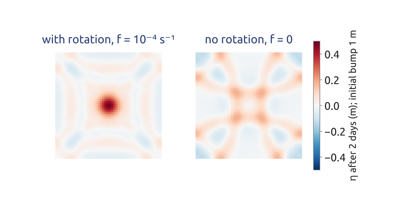
Geostrophic adjustment, BDM1 × DG0 (notebook 08c).

Compatible spaces conserve energy and keep geostrophic balance exactly

(Cotter and Shipton 2012; Vallis 2017, sec. 3.9)

Steady state: ∫ f w·u^⊥ − g div(w) η = ∫ div(w)(fψ − gη) = 0 because div w ∈ V² = DG0, where η is the projection of fψ/g. ψ in CG2, u = perp grad ψ in BDM1 exactly (the de Rham complex CG2 → BDM1 → DG0).

Notebook Shallow water with Firedrake

Notebook 08c (open in Colab · download): rotating shallow water with compatible finite elements.

After 2 days, from a 1 m bump of radius 150 km (deformation radius \(L_d = 99\) km): with and without rotation

1. The equations
2. Compatible spaces
3. Weak form and time stepping
4. Geostrophic adjustment: \(f\) and \(f = 0\) ❗ 4.1
5. A balanced state stays balanced; energy kept to round-off 🧩 5.1

A demo or at home; ❗ 4.1: the bump radius against \(L_d\). Predict, run, explain

Compatible elements in a notebook: energy and balance kept to round-off

(Cotter and Shipton 2012; Rathgeber et al. 2016)

Pedro may run it as a demo, 15 min. Exercise 4.1 (the bump radius against L_d) is mandatory; 5.1 (a 6-hour time step) optional.

What the Firedrake notebooks showed

• 08b: DQ1, one rotation: error 0.089; \(q\) changes only through the boundary; small overshoots at jumps
• 08c: energy change \(2\times10^{-15}\) in two days; a balanced state changes by \(10^{-14}\)
• Adjustment: what stays depends on the size of the bump against \(L_d\)

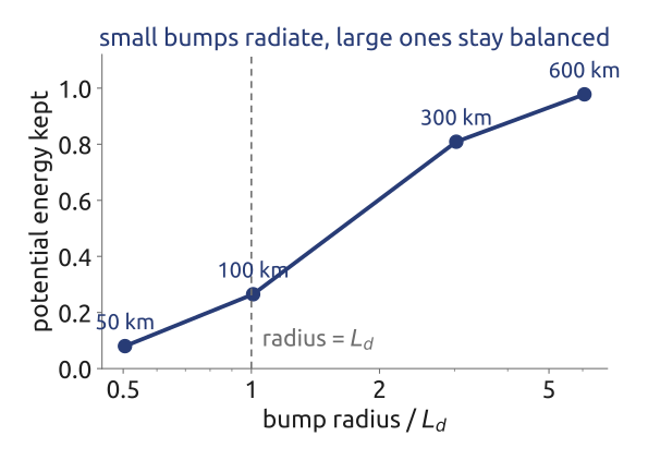
Compatible elements keep the physics of the shallow water equations: energy, balance, waves

(Cotter and Shipton 2012; Vallis 2017, sec. 3.9)

Values from the notebooks (Firedrake 2026.10.0, Docker image). 50 km bumps are also poorly resolved (cells ~40 km).

Gusto: a dynamical core from these pieces

• Gusto: a Python library on Firedrake for compatible finite element dynamical cores (Imperial College London, Met Office, Exeter)
• A test bed for the compatible methods that underpin LFRic, the Met Office’s next model

• Shallow water, Boussinesq, compressible and moist Euler equations; the standard test cases

But: which spaces, and why those?

A dynamical core: a mesh, compatible spaces, the equations in weak form, a time stepper

(Bendall et al. 2020; Shipton et al. 2018) · Code: github.com/firedrakeproject/gusto

Each piece is a lecture of this course. Ask first: which of these boxes did lectures 4–8 build? (The spaces and the time step; the mesh in lecture 9.) Gusto is open source; its examples include all the Williamson test cases.

Compatible spaces: the de Rham complex

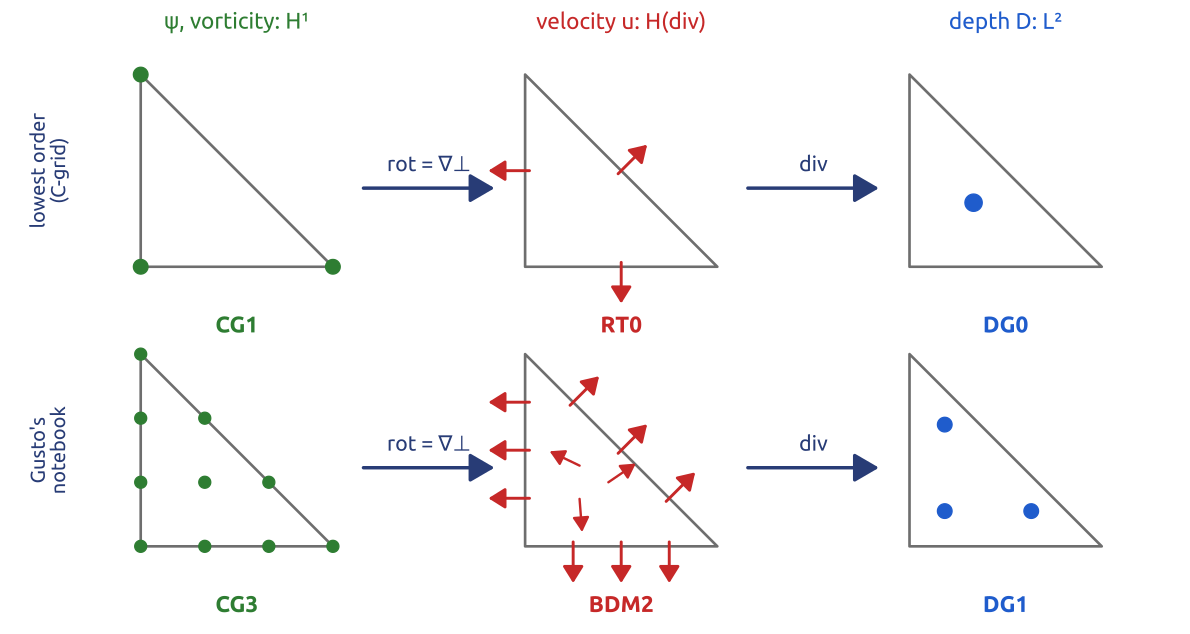
\[H^1 \xrightarrow{\;\nabla^\perp\;} H(\mathrm{div}) \xrightarrow{\;\nabla\cdot\;} L^2, \qquad \nabla\cdot\nabla^\perp = 0\]

• Streamfunction and vorticity in \(H^1\), velocity in \(H(\mathrm{div})\) (normal components across edges), depth in \(L^2\)
• The discrete spaces \(V^0 \to V^1 \to V^2\) keep the identities: \(\nabla\cdot V^1 = V^2\); a discrete \(\nabla^\perp\psi\) has no divergence
• Lowest order: the C-grid on triangles (CG1 → RT0 → DG0); Gusto’s notebook: CG3 → BDM2 → DG1

\(V^0 \subset H^1\) (streamfunction, vorticity), \(V^1 \subset H(\mathrm{div})\) (velocity), \(V^2 \subset L^2\) (depth), as in Cotter & Thuburn 2014

Each variable lives in the space that matches what the equations do to it

(Cotter and Shipton 2012; Cotter and Thuburn 2014; Natale et al. 2016)

Ask first: on the C-grid (lecture 6), where did u and h live, and why? (Normal velocities on the faces, h at the centres: the divergence and the gradient need no averaging.) Vorticity is diagnosed in H1: integral of gamma zeta = minus integral of grad-perp gamma . u, for every test gamma.

Weak form in Gusto (1/2): the fast waves

\[\partial_t\mathbf u + (\zeta + f)\,\mathbf u^\perp + \nabla\!\left(g(D + b) + \tfrac12|\mathbf u|^2\right) = 0, \qquad \partial_t D + \nabla\cdot(D\mathbf u) = 0\]

\(\zeta\): relative vorticity; \(D\): fluid depth; \(b\): height of the orography

The fast part (gravity waves, rotation), linearized about rest, \(D = H + \eta\); tests \(\mathbf w \in H(\mathrm{div})\), \(\phi \in L^2\); the pressure term integrated by parts (no boundary on the sphere):

\[\begin{aligned} \int \mathbf w\cdot\partial_t\mathbf u + f\,\mathbf w\cdot\mathbf u^\perp - g\,{\color{#1f5ccc}(\nabla\cdot\mathbf w)}\,\eta\;dA &= 0\\ \int \phi\,\partial_t\eta + H\,\phi\,{\color{#1f5ccc}\nabla\cdot\mathbf u}\;dA &= 0 \end{aligned}\]

Only the divergence of the velocity appears: \(\mathbf u, \mathbf w \in H(\mathrm{div})\) is enough, and \(\eta \in L^2\) needs no derivative at all

The same linear system as in compatible elements (2/2), now on the sphere

But: and the nonlinear transport terms?

Velocity in \(H(\mathrm{div})\), depth in \(L^2\): exactly the derivatives the fast terms need

(Cotter and Shipton 2012; Shipton et al. 2018)

The full nonlinear terms are in the residual; this linear part is what the implicit solver inverts (next slides). Energy conservation follows with w = H u, phi = g eta (Compatible (2/2)).

Weak form in Gusto (2/2): DG transport

The upwind flux of DG (3/4).

The slow part, transport by the wind, on each triangle \(K\), integrated by parts (DG, this lecture):

\[\int_K \phi\,\partial_t D - \int_K \nabla\phi\cdot\mathbf u\,D + \oint_{\partial K}\phi\,(\mathbf u\cdot\mathbf n)\,\tilde D = 0\]

\(D\): fluid depth (free-surface height minus the orography \(b\)); \(\phi\): test function (as in Cotter & Shipton 2012)

• \(\tilde D\): the upwind value on each edge; depth (and mass) conserved exactly
• Velocity: the vorticity and kinetic-energy terms, also upwinded at the edges (Gusto today; Shipton et al. 2018 transported the potential vorticity)
• Depth: explicit SSP-RK3, two substeps per step (velocity: trapezium rule): limited by the wind, not by the gravity waves

Slow transport: explicit and upwind; fast waves: implicit and compatible

(Shipton et al. 2018; Bendall et al. 2020)

Wind about 40 m/s against gravity waves of 240 m/s: the transport Courant number is six times smaller. LFRic replaced its transport by a flux-form semi-Lagrangian scheme (SWIFT, 2024–25), conservative and stable at large Courant numbers.

One time step: semi-implicit quasi-Newton

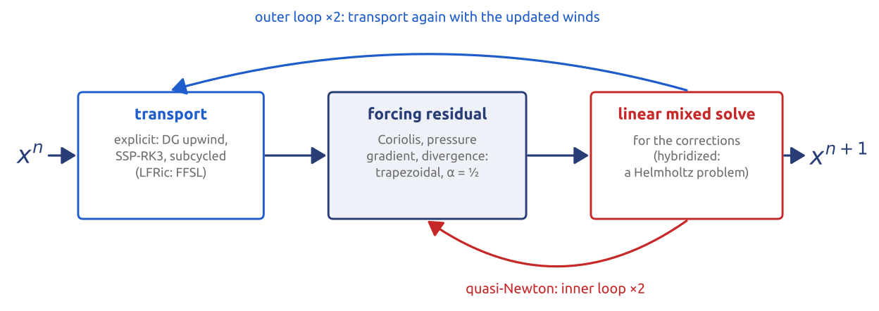
Transport: explicit, subcycled: limited only by the wind

Forcing: implicit, trapezoidal; 2 quasi-Newton iterations, each a linear solve about the rest state: a Helmholtz problem, on a mesh

No CFL for gravity waves: Gusto stable at Courant 5.5 (steps of 4 h); LFRic: up to 10 (20 km, 10 min)

Explicit where it is cheap, implicit where the waves are fast: the structure of all global models

(Melvin et al. 2019; Wood et al. 2014; Bendall et al. 2020)

CFL: lecture 5; Helmholtz problem: lecture 7. Quasi-Newton: the Jacobian is replaced by the linearization about a fixed reference state (H, f), the same every step. The mixed (u, D) system can be hybridized: Lagrange multipliers on the edges leave a smaller, symmetric positive definite problem. ENDGame (the UM) and the IFS have the same structure with semi-Lagrangian transport.

LFRic: GungHo in operation

	UM (ENDGame)	LFRic (GungHo)
Grid	latitude–longitude	equiangular cubed sphere
Waves and forces	finite differences	lowest-order compatible finite elements
Horizontal	C-grid	its finite element equivalent
Vertical	Charney–Phillips	its finite element equivalent
Equations	non-hydrostatic, deep atmosphere	the same
Transport	semi-Lagrangian	flux-form semi-Lagrangian (conservative)
Time step	semi-implicit	semi-implicit

Named after Lewis Fry Richardson

• 2011: the GungHo project begins
• 2013: compatible finite elements chosen
• 2015: the cubed sphere
• 2022: the model runs with full physics
• 2027: first parallel suite
• 2028: the operational model

LFRic: the same staggering as the UM, rebuilt with compatible elements on the cubed sphere

(Melvin et al. 2024; Bendall and Kent 2025); T. Bendall, “Recent progress on the Met Office’s LFRic-Atmosphere model”, PDEs on the Sphere, São Paulo, 2025

Why: no pole (scalability, lecture 9), local conservation, portability to new computers (code generation with PSyclone, as Firedrake’s), modern data assimilation. Timeline from Bendall’s 2025 talk (courtesy of N. Wood). Charney-Phillips: lecture 4. Richardson: lecture 1.

Notebook Gusto: shallow water on the sphere

Notebook 08d (open in Colab · download): a dynamical core in a notebook, shallow water on the sphere with Gusto.

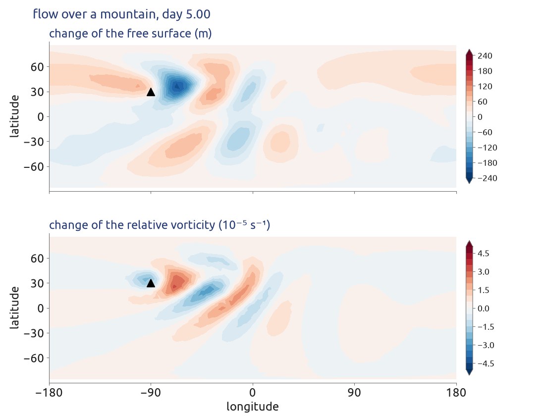
Case 5, five days: change of the free surface and of the vorticity; ▲ the mountain

1. The equations and potential vorticity
2. The mesh, the spaces, the weak form: count the unknowns
3. Case 2: a balanced flow; predict the Courant number
4. Case 5: a mountain in the flow; predict where the waves go
5. Exercises: convergence ❗ 5.1, no rotation ❗ 5.2, another pair of spaces 🧩 5.3

About 3 min of computing (5 with the exercises)

A real dynamical core, step by step: mesh, spaces, equations, time step

(Williamson et al. 1992; Bendall et al. 2020)

A demo or at home. Williamson et al. (1992) cases 2 and 5, after Gusto’s own examples. Install: FEM on Colab, then Gusto with pip (first cell). Tested in the Firedrake Docker image; check it in Colab before the course. The video: over the mountain the column is squashed, zeta + f falls with D (anticyclonic); downstream, beta turns the columns back and forth: a stationary Rossby train, about 60 degrees of longitude per wavelength.

What the Gusto notebook showed

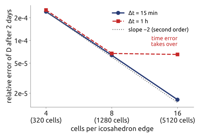
• Case 2 (balanced flow): relative error \(\sim10^{-4}\) after 2 days at a gravity-wave Courant number of 1.4; second order in space: halve the triangles, divide the error by 4
• At 16 cells per edge, steps of 1 h hide that: the time error takes over. Refine space and time together
• Case 5: \(Q = (\zeta + f)/D\) conserved; over the mountain \(\zeta\) falls, downstream \(\beta\) makes a stationary Rossby wave train; without rotation, none
• The spaces matter: the triangular C-grid (\(\mathbf u\) in RT0, \(D\) in DG0) has 60 times the error

A real dynamical core in a notebook: accurate, stable with long steps, and the right waves

(Williamson et al. 1992; Shipton et al. 2018)

Space and time errors: lecture 5. Errors with 15-min steps: 2.4e-4, 6.4e-5, 1.6e-5 for 4, 8, 16 cells per edge; with 1-h steps the 16-cell error stays at 6.5e-5. RT0 x DG0 (Firedrake’s RT1): 4.3e-3 against 6.7e-5 (1-h steps, 8 cells per edge); BDFM1 x DG1 (2:1, Firedrake’s BDFM2) as accurate as BDM2 x DG1. No checkerboard: L_d = 2400 km here (Cotter & Shipton 2012: it shows when L_d is small).

Finite elements in weather and climate models

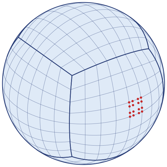
Cubed-sphere mesh; red: the nodes of one spectral element of degree 3.

Model	Centre	Finite elements	Status
LFRic (GungHo core)	Met Office, UK	compatible, lowest order; cubed sphere	operational from 2028
KIM	KIAPS, Korea	spectral elements; cubed sphere	Korea’s global forecast model
CAM-SE, E3SM	NCAR, US DOE	spectral elements (HOMME); cubed sphere	climate models
NEPTUNE (NUMA core)	US Navy, NRL	spectral elements on any quadrilateral mesh	the US Navy’s model (closed code)
ClimaAtmos	CliMA, Caltech	spectral elements in the horizontal; cubed sphere	climate model

LFRic does not use Firedrake: it is Fortran 2003, with the science code kept apart from the parallel code (PSyKAl layers), and the code generator PSyclone (STFC Hartree Centre) writes the parallel layer. Gusto, in Python on Firedrake, is the test bed of its numerics.

Element methods scale: each element talks only to its neighbours

(Adams et al. 2019; Choi and Hong 2016; Dennis et al. 2012; Kelly and Giraldo 2012; Yatunin et al. 2025) · NEPTUNE fact sheet · ClimaAtmos

LFRic: first parallel suite 2027, operational 2028 (Bendall’s talk, 2025). Spectral elements: continuous Galerkin with high-order Lagrange polynomials at GLL nodes and a diagonal (lumped) mass matrix (Taylor & Fournier 2010).

Finite elements and DG in ocean models

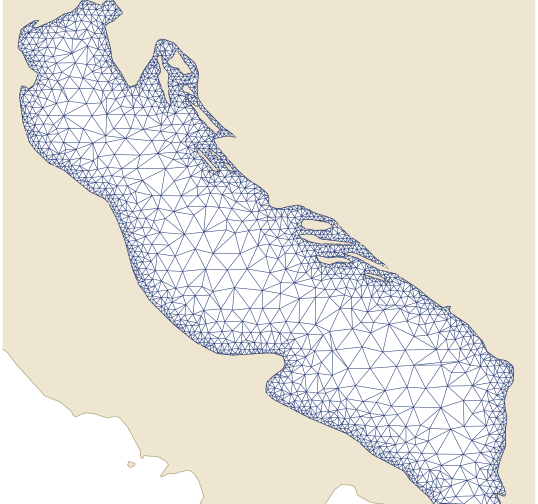
Schematic: a mesh of the Adriatic refined towards the coast, not a model’s mesh.

• Rare in the ocean: global and climate models use finite differences or finite volumes on structured grids (NEMO, MOM, POP, HYCOM): 10 of the 11 models of OMIP-2

Model	Finite elements	Use
ADCIRC (US)	continuous Galerkin, triangles	NOAA’s global tide and surge
SCHISM (US)	hybrid finite element–finite volume	NOAA, Atlantic coast
SHYFEM (CNR-ISMAR, Italy)	finite elements, triangles	Adriatic, Venice lagoon
FESOM 1.4 (AWI)	continuous Galerkin	CMIP6; FESOM2: finite volumes
Fluidity (Imperial College)	adaptive tetrahedra	research
SLIM (UCLouvain), Thetis	DG	research

But: continuous elements need a global solve and stabilized advection (FESOM2 moved to finite volumes, three times faster); DG, local and conservative, is so far in research codes

Finite elements are rare in the ocean: they live on the coast, where meshes follow the shore

(Tsujino et al. 2020; Cirano et al. 2025; Danilov et al. 2017; Kärnä et al. 2018) · NOAA STOFS

OMIP-2 (Tsujino et al. 2020, Table 1): 11 models, 10 on structured B or C grids; the exception, FESOM 1.4, was AWI’s CMIP6 ocean. Operational coastal finite elements: ADCIRC (NOAA STOFS-2D-Global), SCHISM (STOFS-3D-Atlantic), SHYFEM (Adriatic, Venice; Cirano et al. 2025). Thetis uses the same Firedrake as today’s notebooks.

Research: DG on Voronoi meshes

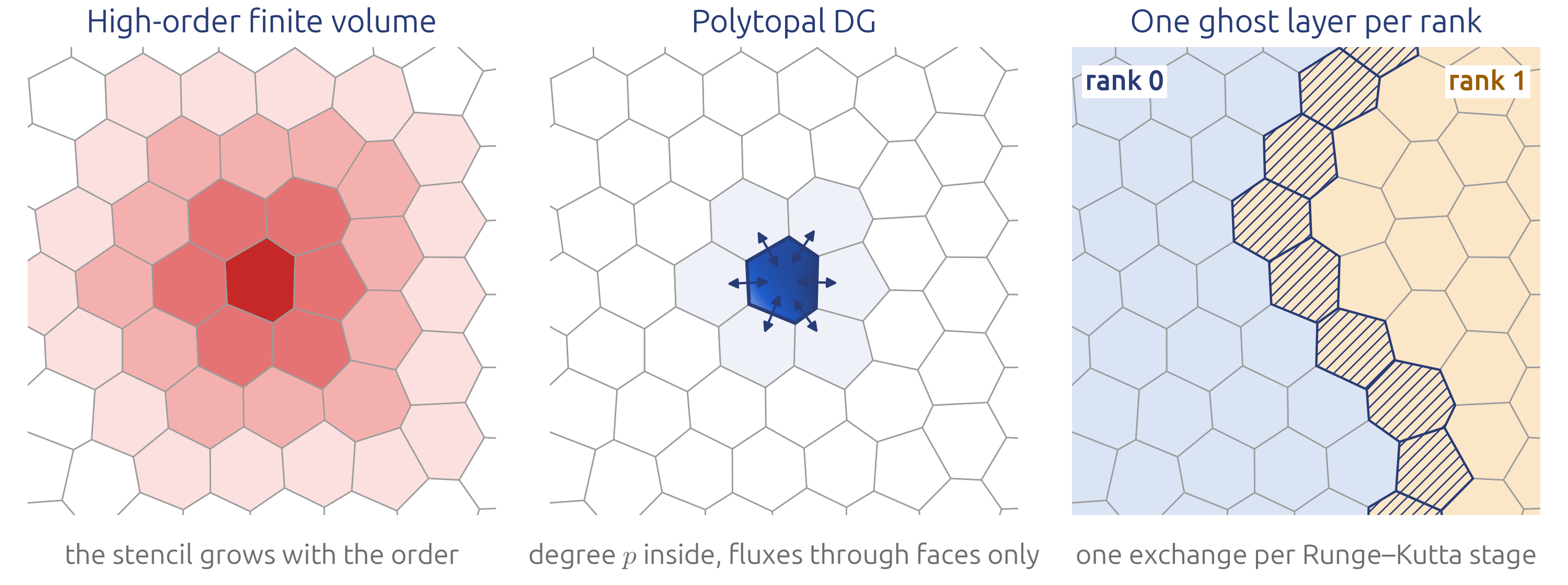
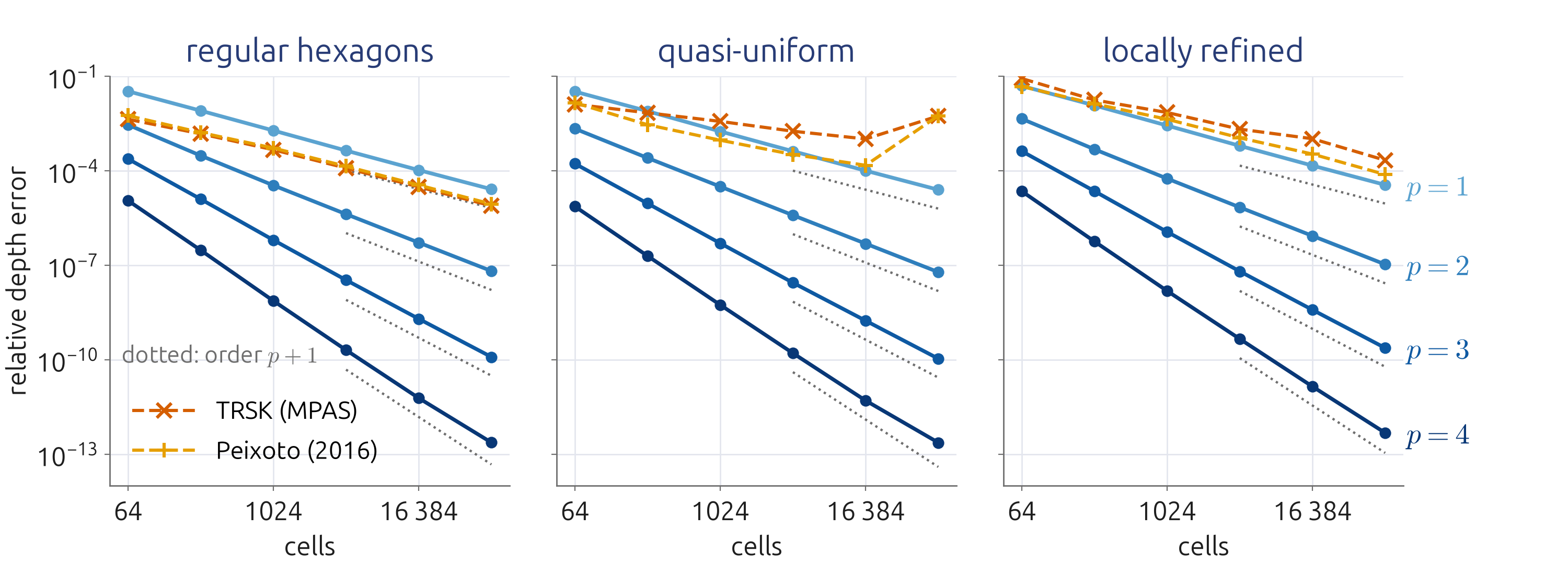
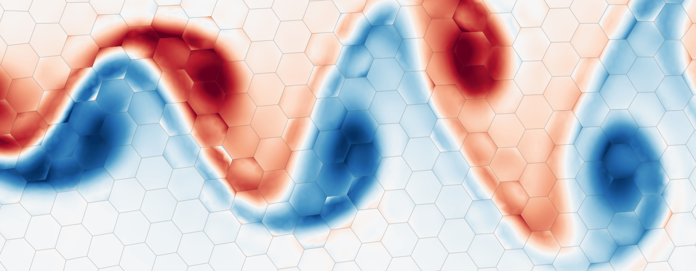
• Polytopal DG (PolyDG, with MOX) for the rotating shallow water equations on Voronoi meshes, as in MPAS
• Order \(p + 1\) on every mesh, also irregular and locally refined ones, where the finite volumes of MPAS (TRSK) lose accuracy

Left: an unstable jet, relative vorticity (red positive, blue negative) at day 14; DG of degree \(p = 4\) on a Voronoi mesh of 4096 cells, the cell edges in grey

Local and high order on the meshes of operational models: an open research direction

Peixoto, Alves, Fumagalli & Antonietti, M4E 2026 talk; paper in preparation (the jet: its graphical abstract)

Pedro’s own work (M4E 2026, Politecnico di Milano). Left: why DG is local; right: convergence against TRSK (MPAS) on regular, quasi-uniform and locally refined meshes. Bottom: the jet, a crop of the paper’s graphical abstract (bi-periodic plane, the coarse cells of the locally refined mesh, southern jet rotated by 180°).

Extra A vertical slice with Gusto

Notebook 08e (open in Colab · download), not done in class: the compressible Euler equations in an \(x\)–\(z\) slice.

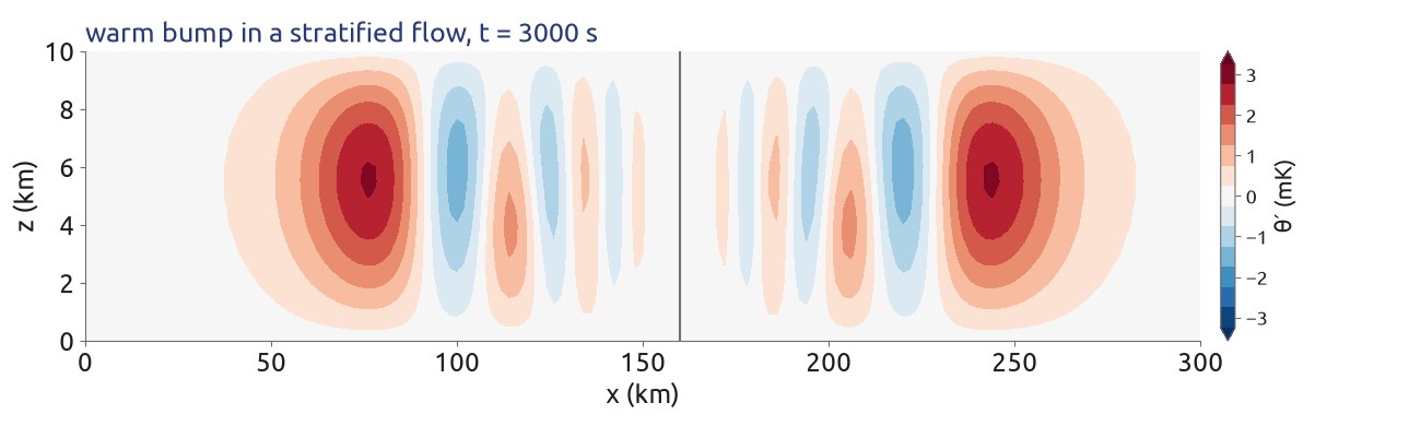
Skamarock & Klemp (1994): a warm bump of 0.01 K in a wind of 20 m/s, \(N = 0.01\) s⁻¹, 3000 s; \(\theta'\) in mK, grey: the centre carried by the wind

• The same compatible spaces, extruded: \(u\) on the sides of each cell, \(w\) on top and bottom, \(\rho\) inside; \(\theta\) with \(w\) (Charney–Phillips)
• The bump splits into internal gravity waves; the long ones lead

• Within a few per cent of linear theory; stable at a sound-wave Courant number of 4
• Exercises: hydrostatic or not ❗ 4.1, the time step 🧩 4.2

A non-hydrostatic dynamical core in a notebook, with the vertical staggering of ENDGame and LFRic

(Skamarock and Klemp 1994; Bendall et al. 2020)

An extra, not done in class: for students who want the vertical. About 3 min of computing (4 with the exercises). The vertical numerics come back in lecture 9 (the standard tests: gravity waves, Straka, Schär).

Key points

1. Weak form: multiply by a test function \(v\), integrate, by parts: \(\int u'v'\,dx = \int fv\,dx\), only first derivatives
2. Galerkin: \(u_h = \sum_j U_j\ell_j\), tested with every \(\ell_i\): \(SU = F\); hats on a uniform mesh give the centred finite-difference Laplacian
3. DG: a polynomial of degree \(p\) in each element; elements meet only through a numerical flux at the faces, upwind \(\hat F = c\,u^-\)
4. DG with \(p = 0\) is upwind finite volumes; error \(\sim h^{p+1}\) for smooth fields; Courant limit about \(1/(2p+1)\) with SSP-RK3
5. Godunov: linear schemes of high order overshoot at jumps; DG only in a narrow band
6. Compatible elements, \(\nabla\cdot V^1 = V^2\): the C-grid on any mesh; energy and geostrophic balance kept exactly
7. Firedrake: the weak form is the code; Gusto builds dynamical cores on it, a test bed for the compatible methods of LFRic (Met Office)
8. In use: spectral elements (KIM, CAM-SE, E3SM, NEPTUNE, ClimaAtmos), compatible (LFRic); coastal ocean models

Notebooks:
08a (open in Colab · download): DG in 1D · 08b (open in Colab · download): DG in 2D with Firedrake
08c (open in Colab · download): compatible shallow water · 08d (open in Colab · download): Gusto on the sphere
08e (open in Colab · download): a vertical slice with Gusto

Finite elements: local, high order, on any mesh, and still conservative

Reading: (Durran 2010, secs. 6.5–6.6; Hesthaven and Warburton 2008; Cockburn 2003; Cotter and Shipton 2012)

Next lecture’s warm-up asks about these. Each Firedrake and Gusto notebook has one mandatory exercise (Pedro, 2026-10-23; Colab install still untested). Next: which mesh for the whole sphere, at kilometre scales? How do operational models assemble these pieces (lecture 9), and what do AI models change (lecture 10)?