Modern weather, ocean and climate models
Atmosphere and Ocean Dynamics, Lecture 9: notes
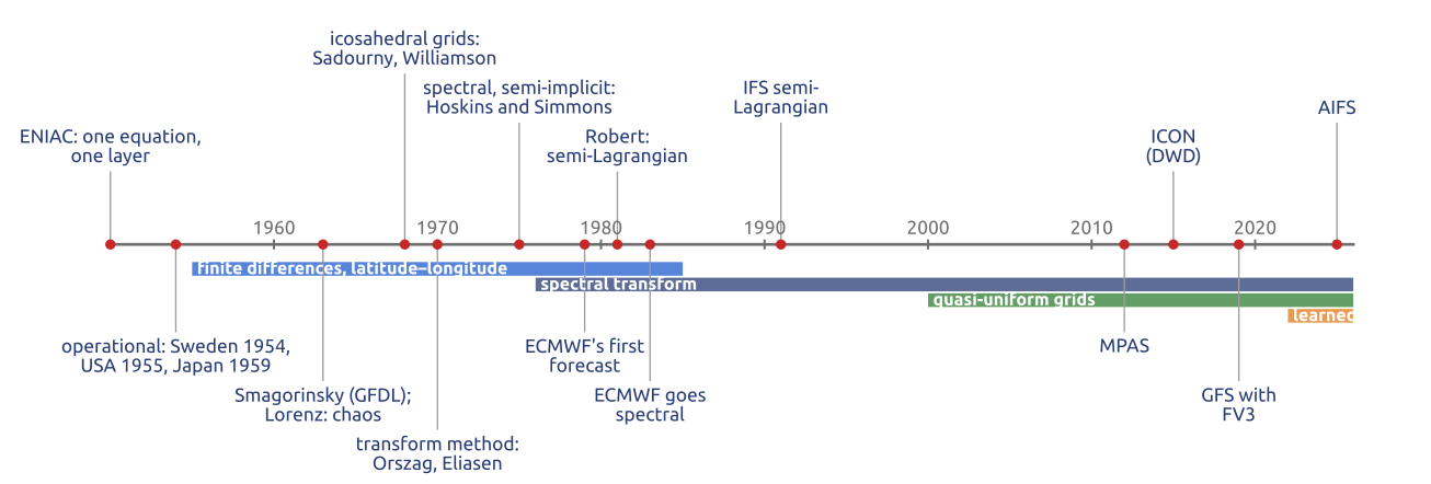
How today’s weather and ocean models came to be, from the 1950 forecast onwards. These notes discuss the first general circulation models and Lorenz’s limit of predictability, hence ensembles; the pole problem, and semi-Lagrangian and semi-implicit steps; the spectral era and its scaling limit; the new models on quasi-uniform grids; the choices in the vertical (staggering, the treatment of sound waves, sponges, vertical coordinates); standard tests and intercomparisons; and ocean models since Bryan’s of 1969, from a rigid lid to a free surface and from \(z\)-levels to isopycnal, hybrid and unstructured grids.
1 1950: one equation, one layer
The first numerical forecast that worked integrated one equation for one layer, the barotropic vorticity equation \[ \frac{\partial\zeta}{\partial t} + J(\psi, \zeta + f) = 0, \qquad \nabla^2\psi = \zeta , \] with \(\zeta\) the relative vorticity, \(\psi\) the streamfunction, \(f\) the Coriolis parameter and \(J(\psi, q) = \psi_x q_y - \psi_y q_x\) the advection of \(q\) by the non-divergent wind. At every step the advection gives the tendency of the vorticity, and a Poisson problem gives back the streamfunction. The forecast of Charney et al. (1950) ran on the ENIAC at Aberdeen in 1950, with centred finite differences on a polar stereographic grid of 736 km at the North Pole, and time steps of 3 hours; a 24-hour forecast took about 24 hours of computing, most of it in handling punched cards (Lynch 2008). The equation has no gravity waves, so, unlike Richardson’s forecast of 1922, the initial state needed no balancing. The slide compares the computed 24-hour change of the 500 hPa height of 30 January 1949 with the observed one (Charney et al. (1950), Fig. 3c; CC BY 4.0). One level of one variable, however, leaves out the vertical, temperature, moisture, gravity waves and the whole globe.
2 1950–1975: towards the general circulation
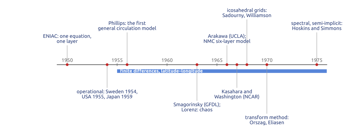
In twenty years the models grew from one equation for one layer to general circulation models (Figure 1). Operational barotropic forecasts started in Sweden in 1954, the USA in 1955 and Japan in 1959 (Randall et al. 2019). Phillips (1956) integrated a two-level model for a month of the general circulation: the first climate model. In the 1960s the primitive equations came back, now with better initial states and smoothing: Smagorinsky’s model at GFDL (SMAGORINSKY 1963), Mintz and Arakawa’s at UCLA (with Arakawa’s energy-conserving Jacobian and staggered grids), Kasahara and Washington’s at NCAR (KASAHARA and WASHINGTON 1967), and the six-layer primitive-equation model of the US National Meteorological Center, operational from 1966 (Shuman and Hovermale 1968). All used finite differences on latitude–longitude grids.
3 1963: Lorenz and the limits of prediction
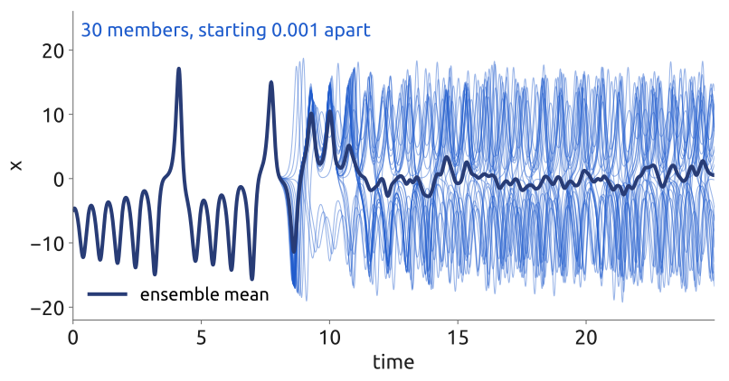
Lorenz (1963) showed with a system of three equations, a truncated model of convection, that the solutions of some deterministic systems depend so strongly on their initial state that two very close states give, after a while, unrelated solutions (Figure 2). The atmosphere behaves this way: errors in the initial state grow fastest at small scales and spread to the large ones, and the limit of deterministic predictability of the weather is about two weeks (Kalnay 2003, Ch. 6). Since the initial state always has errors, one forecast is not enough. An ensemble runs the model from many initial states, all consistent with the observations, often with perturbed physics too; the spread of the members says how much to trust the forecast, and their mean is often better than any single member. ECMWF’s ensemble has 50 perturbed members and a control. Each member, though, is a full model, which needs a grid on the sphere.
4 Finite differences and the pole problem
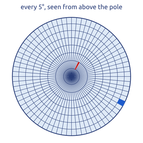
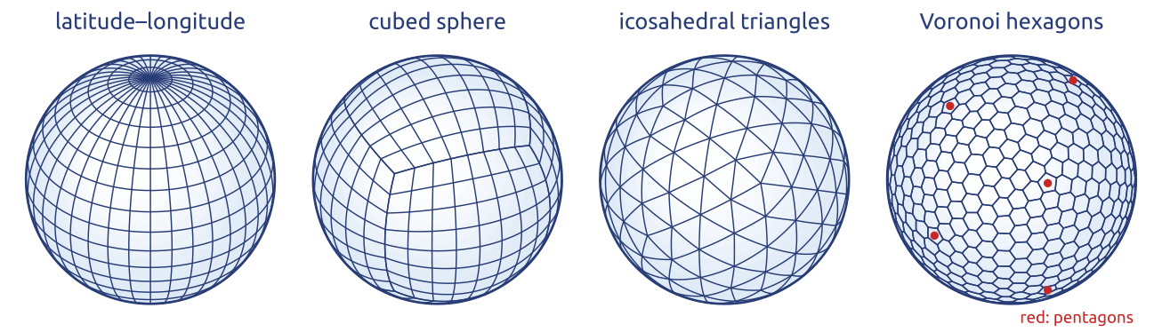
From the 1960s to the 1980s most global models used finite differences on latitude–longitude grids, as Richardson had: GFDL, UCLA (with Arakawa’s staggered grids), NCAR, NMC. On such a grid with spacing \(\Delta\lambda\) the east–west distance between points is \[ \Delta x = a\cos\varphi\,\Delta\lambda , \] with \(a\) the radius of the Earth and \(\varphi\) the latitude: it goes to zero at the poles, where the meridians meet and the cells become thin wedges (Figure 3). With an explicit scheme the CFL condition requires \(\Delta t \le \Delta x/c\) in every cell, for the fastest waves \(c\), so the cells next to the poles set the time step of the whole model. The fixes of the time were polar filters, which remove the short east–west waves at high latitudes, and reduced grids with fewer points along the latitude circles near the poles (Staniforth and Thuburn 2012; Williamson 2007).
5 In class: the pole problem in numbers
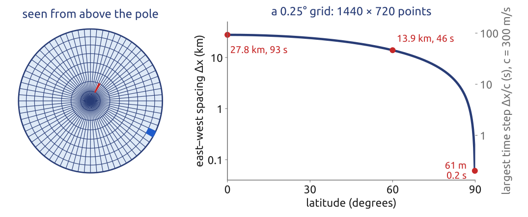
Exercise 1 — The pole problem. A latitude–longitude grid with a spacing of \(0.25^\circ\) (\(1440\times720\) points). Compute the east–west spacing \(\Delta x = a\cos\varphi\,\Delta\lambda\) at the equator, at \(60^\circ\)N and in the last row, \(89.875^\circ\)N, and the largest stable explicit time step \(\Delta t = \Delta x/c\) for gravity waves with \(c = 300\) m/s.
Data: \(a = 6371\) km, \(\Delta\lambda = 0.25^\circ = 4.36\times10^{-3}\) rad.
To hand in. A quasi-uniform grid with the same number of columns: its mean spacing \(\sqrt{4\pi a^2/N}\) and its time step. How many columns does a global grid of 1 km need?
6 What the exercise showed
With \(a\,\Delta\lambda = 6371\ \text{km}\times4.36\times10^{-3} = 27.8\) km, the east–west spacing is 27.8 km at the equator, \(27.8\cos60^\circ = 13.9\) km at \(60^\circ\)N and \(27.8\cos89.875^\circ = 61\) m in the last row; the largest explicit steps for \(c = 300\) m/s are 93 s, 46 s and 0.2 s (Figure 4). The last row near the pole sets the step of the whole model: more than four hundred times shorter than the equator alone would allow. A quasi-uniform grid with the same \(1440\times720 = 1.04\times10^6\) columns has a mean spacing \(\sqrt{4\pi a^2/N} = 22\) km and a step of 74 s. A global grid of 1 km needs \(4\pi a^2/(1\ \text{km})^2 = 5.1\times10^8\) columns.
7 Semi-Lagrangian: follow the air back
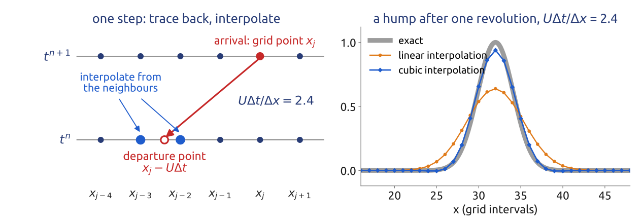
The semi-Lagrangian method computes advection along trajectories. For \(\partial_t u + U\partial_x u = 0\), with \(U\) the wind speed, the value at the grid point \(x_j\) at \(t^{n+1}\) is the value at the departure point \(\tilde x_j = x_j - U\Delta t\) at \(t^n\), which in general lies between grid points and is interpolated. With linear interpolation, \[ u_j^{n+1} = u^n(\tilde x_j) \approx (1 - \alpha)\,u^n_{j-p} + \alpha\,u^n_{j-p-1}, \] where \(p\) is the integer part of the Courant number \(U\Delta t/\Delta x\) and \(\alpha = (x_{j-p} - \tilde x_j)/\Delta x \in [0, 1)\) its fractional part. For \(p = 0\) this is the upwind scheme; for any \(p\) the von Neumann amplification factor satisfies \[ |A|^2 = 1 - 2\alpha(1 - \alpha)(1 - \cos k\Delta x) \le 1 , \] so the scheme is stable for every Courant number (Durran 2010, Sect. 7.1.1). This does not contradict the CFL condition: the backward trajectory places the interpolation stencil, the numerical domain of dependence, around the true one, wherever it is (Figure 5). Linear interpolation damps the short waves strongly; models use cubic interpolation. With a variable wind the departure point is found by integrating the trajectory backwards, usually by a few fixed-point iterations. Interpolation does not conserve mass exactly; conserving variants exist.
Combined with a semi-implicit treatment of the gravity waves, the semi-implicit semi-Lagrangian (SISL) scheme, introduced by André Robert in 1981, allows steps of several minutes at 9 km (Staniforth 1997).
8 The spectral era (1970s–today)
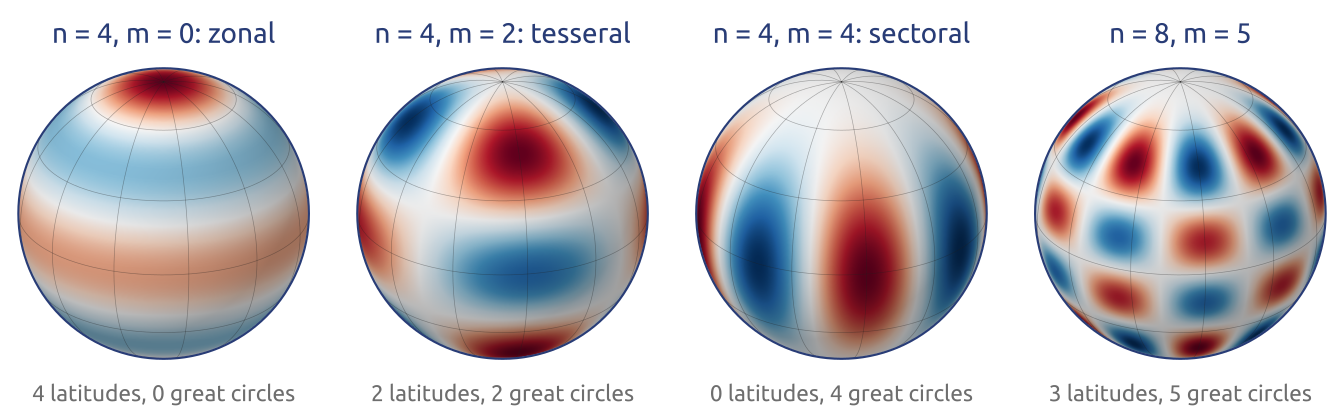
Spherical harmonics \(Y_n^m\), the eigenfunctions of the Laplacian on the sphere, are smooth at the poles, and a triangular truncation has the same resolution everywhere: a spectral model has no pole problem (Figure 6). Two steps made spectral models practical. The transform method (Orszag 1970; Eliasen et al. 1970) computes derivatives exactly in spectral space and products on a grid, which avoids the costly interaction coefficients of a purely spectral product. Multi-level, semi-implicit spectral models (Bourke 1974; HOSKINS and SIMMONS 1975) treat the gravity waves implicitly: in spherical harmonics the Laplacian is diagonal, \(\nabla^2 Y_n^m = -n(n+1)Y_n^m/a^2\), so the Helmholtz problem of the semi-implicit step is a division per coefficient (a small matrix over the levels, for many levels). ECMWF’s first operational forecast, in 1979, came from a grid-point model; its spectral model went into operations in 1983 (Simmons et al. 1989), and the semi-Lagrangian scheme was added in 1991 (Ritchie et al. 1995), with steps of many minutes. For forty years spectral transforms carried most global forecasts (Williamson 2007).
9 Spectral models today
Spectral models with semi-implicit semi-Lagrangian steps are still operational in several centres:
| Model (centre) | Resolution | Levels | Time step |
|---|---|---|---|
| IFS (ECMWF, Europe) | about 9 km (TCo1279) | 137 | SISL |
| YHGSM (NUDT, China) | about 15 km (TL1279) | 137 | SISL |
| HGFM / BFS (IITM, India) | about 6.5 km (TCo1534) | 64 | SISL |
| BAM (CPTEC/INPE, Brazil) | about 20 km | 96 | semi-implicit, Eulerian or SL |
| GSM (JMA, Japan) | about 13 km (TQ959) | 128 | SISL |
| ARPEGE (Météo-France), stretched | about 7 km over France (T1198) | 105 | SISL |
| GFS (NOAA, USA), 1980–2019 | about 13 km (TL1534) | 64 | SISL |
| AROME (Météo-France), limited area | 1.3 km (bi-Fourier) | 90 | SISL |
| EC-Earth3 (Europe), climate | about 80 km (TL255) | 91 | SISL |
TCo is a cubic truncation on an octahedral reduced Gaussian grid (four grid points per shortest wave), TL a linear one (two points per wave), TQ a quadratic one (three); SISL is semi-implicit semi-Lagrangian, SL semi-Lagrangian. The Global Spectral Model of the Japan Meteorological Agency has run at TQ959 with 128 levels since March 2023 (Japan Meteorological Agency 2024; Yonehara et al. 2025). Météo-France’s ARPEGE is spectral on a stretched sphere, finest over France (in 2016 T1198 with a stretching factor 2.2: about 7 km over France, 33 km over the South Pacific), and its limited-area model AROME uses a Fourier series in both horizontal directions (bi-Fourier), made periodic by an extension zone, at 1.3 km (Courtier and Geleyn 1988; Météo-France 2016; Seity et al. 2011). In climate, the European model EC-Earth3 uses the IFS at TL255 with 91 levels, coupled to the ocean model NEMO (Döscher et al. 2022). The Brazilian Global Atmospheric Model is described by Figueroa et al. (2016), India’s High-Resolution Global Forecast Model, the basis of the Bharat Forecast System, by Krishna et al. (2025); YHGSM is the spectral model of the National University of Defense Technology (Jiang et al. 2021). The US GFS, spectral since August 1980 (Sela 1980), left the spectral core in June 2019 for the finite-volume cubed-sphere core FV3. The entries for YHGSM and GFS follow Pedro Peixoto’s BRICS 2026 talk, which called this combination “the state of the art of the millennium”.
10 The scalability problem
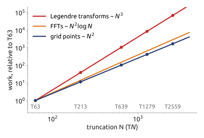
A forecast must finish in about an hour, on machines of \(10^5\)–\(10^6\) cores. For a triangular truncation \(N\) on a quadratic grid there are about \(N^2/2\) coefficients and about \(1.5N\) latitudes, so a Legendre transform of one field costs about \(0.75N^3\) operations, while the FFTs cost \(O(N^2\log N)\) and the grid has \(O(N^2)\) points (Williamson 2007) (Figure 7). Halving the spacing (doubling \(N\)) multiplies the grid points by 4 and the Legendre work by 8. Fast Legendre transforms, which exploit the structure of the associated Legendre functions, reduce this cost at high resolution (Wedi et al. 2013). The harder problem is communication: every spectral coefficient depends on every grid point, so each transform needs data from the whole globe, exchanged across the whole computer at every step. The large linear solves of semi-implicit grid-point models have the same problem. Local methods, which exchange data only with neighbouring cells, avoid it (Bauer et al. 2021). This is the reason for a new generation of models.
11 The kilometre scale
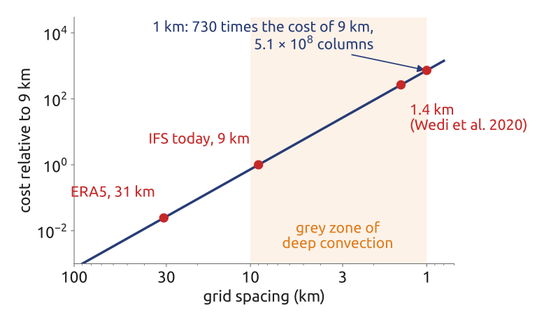
Halving the grid spacing \(\Delta x\) multiplies the number of columns by 4 and, through the CFL condition, halves the time step: the cost of a forecast grows like \(\Delta x^{-3}\), more if the number of levels grows too. From 9 km to 1 km the cost is multiplied by about \(9^3 \approx 730\), and a global 1 km grid has \(5.1\times10^8\) columns (Figure 8). At a few kilometres deep convection starts to be resolved, but not well enough to drop its parameterization: the “grey zone”. Wedi et al. (2020) ran the IFS globally at 1.4 km for a four-month simulation. The obstacle is as much the computer as the arithmetic: weather and climate codes reach about 5% of the peak speed of today’s processors, limited by memory access and communication (Bauer et al. 2021). Hence GPUs and local stencils, as in the Met Office’s LFRic, designed for scalability (Adams et al. 2019).
12 Three answers to the pole problem
Spectral transforms. Spherical harmonics have no pole problem: the resolution is uniform over the sphere. The transforms are done on a Gaussian grid, today the octahedral reduced Gaussian grid of ECMWF’s IFS; the Legendre transforms grow costly at high resolution and need global communication.
Long time steps. Semi-implicit schemes treat the terms responsible for the fast gravity waves implicitly (a Helmholtz problem at every step), so that these waves do not limit the step; semi-Lagrangian schemes follow the flow back to the departure point, so that advection does not limit it either. Together they allow steps much longer than an explicit Eulerian scheme: the IFS and the Met Office’s ENDGame core.
Quasi-uniform grids. Cells of nearly the same size everywhere: the cubed sphere (the six faces of a cube projected onto the sphere), icosahedral triangles, and their duals, Voronoi hexagons with 12 pentagons (Figure 9). There is no pole; the price is that the grids are not orthogonal coordinate systems, and the numerical methods must work on general cells (Staniforth and Thuburn 2012; Williamson 2007). In short: change the basis, the time step, or the grid.
13 The new generation: quasi-uniform grids
Quasi-uniform grids are an old idea: icosahedral grids were used in 1968 for the barotropic vorticity equation (SADOURNY et al. 1968; WILLIAMSON 1968), but they were not competitive then with latitude–longitude grids and, from the 1970s, with spectral models (Figure 10). Since about 2000, with the scalability problem, they returned: the cubed sphere (FV3, LFRic), icosahedral triangles (ICON), Voronoi grids (MPAS, and Brazil’s MONAN, built on it). The methods on them are local, finite volumes and finite elements, with communication only between neighbouring cells (Staniforth and Thuburn 2012). No grid on the sphere is perfect, though: each model trades uniformity, orthogonality and the placement of the variables differently.
14 Grids on the sphere
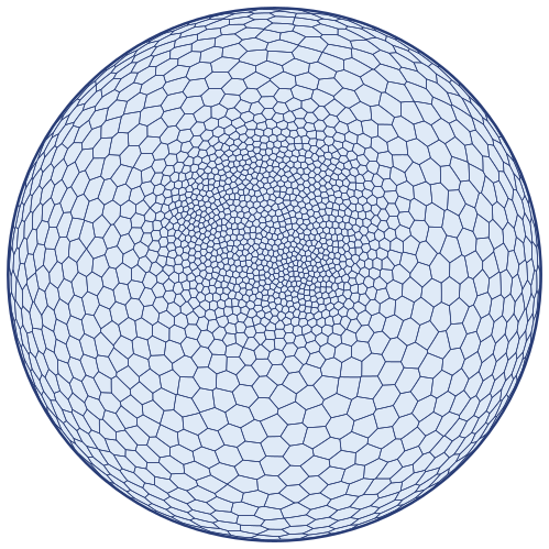
A grid like those of MPAS and MONAN can be built in a few lines of Python, in six steps: Delaunay triangulations and their dual Voronoi diagrams in the plane; on the sphere, where the convex hull of the points gives the Delaunay triangulation (six points make a cube); icosahedral grids, by subdividing the twenty triangles of an icosahedron; Lloyd’s iterations, which move each generator to the centroid of its Voronoi cell and turn random points into a regular grid; local refinement over the Alps, with a density function \(\rho\); and the explicit time step set by the smallest cell, compared with the pole problem. A question to predict before computing: how much smaller do the cells get where the density is 256 times larger? Ringler et al. (2011) describe such variable-resolution grids for the shallow water equations.
15 Centroidal Voronoi grids and refinement
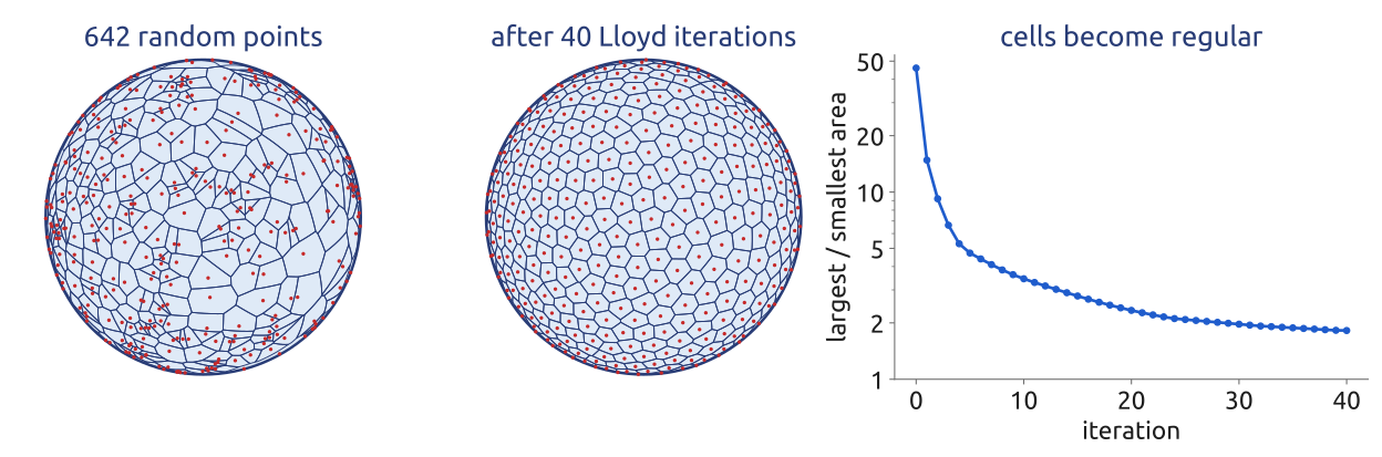
An icosahedron subdivided \(n\) times has \(10\cdot4^n + 2\) vertices: the \(10\cdot4^n + 2\) cells of its dual Voronoi grid are all hexagons except 12 pentagons, at the vertices of the icosahedron (by Euler’s formula a grid of hexagons and pentagons on the sphere needs exactly 12 pentagons). Lloyd’s iterations turn 642 random points, whose cells differ in area by a factor of 46, into a centroidal Voronoi grid, each generator at the centroid of its cell, with a ratio under 2 after 40 iterations (Figure 12). With a density \(\rho\), the spacing of a centroidal Voronoi grid on a surface scales as \(\Delta x \propto \rho^{-1/4}\) (Ringler et al. 2011): a density 256 times larger gives cells 4 times smaller. The smallest cell then sets the explicit time step: refinement puts the small cells where they are wanted, and pays for them everywhere in the step. The same horizontal grids carry the vertical columns of the model; a grid of 15 km has about 2.27 million cells, and with tens of levels and several variables one state holds about \(10^9\) numbers.
16 Where the variables sit
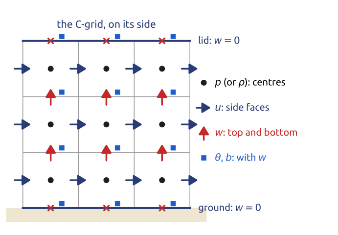
As in the horizontal, the placement of the variables matters in the vertical (Figure 13). The natural grid of a vertical slice is the C grid turned on its side: the pressure (or density) at the cell centres, the horizontal velocity \(u\) on the side faces, the vertical velocity \(w\) on the top and bottom faces, so that the divergence and the pressure gradient need no averaging, and \(w = 0\) is imposed exactly on the faces at the ground and at the lid. Where should the potential temperature \(\theta\), or the buoyancy \(b\), go? It acts on \(w\), through the buoyancy term of the vertical momentum equation, so its natural place is with \(w\): the Charney–Phillips placement. The lowest-order compatible finite elements of Gusto and LFRic place their variables exactly so (Melvin et al. 2019). A slice model in vorticity–streamfunction form keeps \(\psi\), the vorticity of the slice \(\xi\) and \(b\) at the same points: having eliminated the pressure, it needs no staggering.
17 Lorenz and Charney–Phillips grids
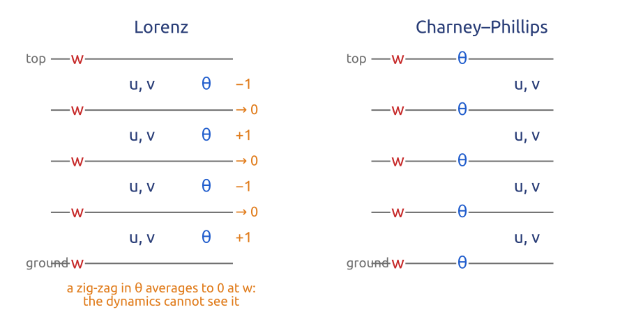
In a column of model layers there are two common placements (Figure 14). The Lorenz grid keeps \(\theta\) at the layer centres with the horizontal winds \(u\), \(v\), and \(w\) at the interfaces; \(\theta\) must then be averaged to the interfaces where the buoyancy acts on \(w\). A zig-zag of \(\theta\) from layer to layer (\(+1, -1, +1, -1\)) averages to zero at every inner interface: the dynamics does not feel it, a computational mode, as the checkerboard of the A grid in the horizontal. The Charney–Phillips grid puts \(\theta\) with \(w\) at the interfaces, where the buoyancy is used. Holdaway et al. (2013) compare the two: the Charney–Phillips grid represents waves and potential vorticity better; the Lorenz grid is simpler for conservation and behaves better in some respects with the boundary layer. The choice is still debated: the Met Office uses the Charney–Phillips grid, ECMWF a variant of the Lorenz grid.
18 Each step: a Poisson problem, or fast sound
The Boussinesq and the anelastic equations have no sound waves: the pressure is whatever keeps the flow (mass-weighted, for anelastic) divergence-free, and it comes from an elliptic problem at every step, as the streamfunction did in the 1950 forecast, or \(\nabla^2\psi = \xi\) in a vorticity–streamfunction slice. Non-hydrostatic weather models (WRF, MPAS, ICON, the Met Office’s Unified Model) solve the compressible equations instead, which carry sound waves at about 340 m/s. Their layers near the ground are a few tens of metres thick while the horizontal spacing is kilometres, so a sound wave travelling vertically would force a tiny explicit step: \[ \Delta t \le \frac{\Delta z}{c_s} = \frac{20\ \text{m}}{340\ \text{m/s}} \approx 0.06\ \text{s}, \] with \(\Delta z\) the thickness of a layer near the ground and \(c_s\) the speed of sound. Hydrostatic models have no vertically travelling sound waves: the hydrostatic approximation filters them. Non-hydrostatic models treat the vertical implicitly: horizontally explicit, vertically implicit (HEVI), or by splitting the fast acoustic modes from the slow ones with small steps, implicit in the vertical (split-explicit, as in WRF and MPAS) (Klemp et al. 2007). An implicit step in one column of \(J\) levels is one tridiagonal solve, \(O(J)\) operations, and the columns are independent of each other, which suits parallel computers (Durran 2010). Semi-implicit models treat the fast waves implicitly in all directions, at the price of a three-dimensional Helmholtz problem every step (the IFS, Gusto). Somewhere there is always an elliptic or implicit solve: the price of fast waves.
19 The top of the model: let the waves out
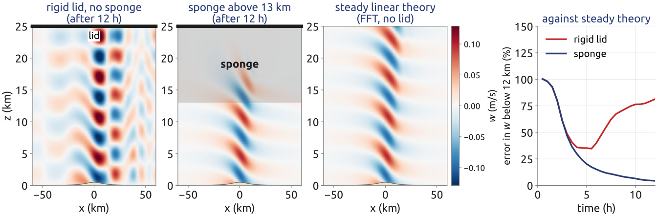
A model’s domain ends somewhere above, usually with a rigid lid. Mountain waves, and the waves sent up by convection, carry energy upwards; at a lid they reflect and come back down, and the radiating solution becomes a standing pattern that has nothing to do with the real atmosphere, which has no lid. Models therefore add a sponge layer in their top part: a Rayleigh damping, \(-\gamma(z)\,\xi\) and \(-\gamma(z)\,b'\) added to the equations for the vorticity of the slice \(\xi\) and the buoyancy perturbation \(b'\), with a rate \(\gamma(z)\) that is zero below the sponge and grows smoothly towards the lid. The waves enter it and fade before they can return. The layer must be deep (at least about a vertical wavelength) and gentle: a damping that switches on too abruptly, or a layer too thin, reflects the waves itself (Klemp and Lilly 1978; Klemp et al. 2008). In a linear slice model of a wind of 10 m/s over a 100 m ridge, the error after 12 h is 81% with the lid alone and 4% with a sponge in the top 12 km (Figure 15). The sponge is a piece of numerics with no physics in it: it stands for the infinite atmosphere above the model.
20 Vertical coordinates
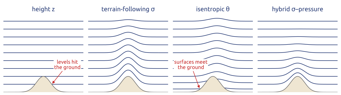
A model must choose the surfaces on which it stores its variables in the vertical (Figure 16).
- Height \(z\). Simple; the horizontal pressure gradient is computed exactly on level surfaces. But the levels cut through mountains, which are then represented by steps (or cut cells).
- Terrain-following \(\sigma\), for example \(\sigma = (z - z_s)/(z_{\mathrm{top}} - z_s)\) with \(z_s\) the height of the ground and \(z_{\mathrm{top}}\) of the lid (Gal-Chen and Somerville 1975), or \(\sigma = p/p_s\) with \(p_s\) the surface pressure. The ground is a coordinate surface, and the coordinate is smooth over mountains; but over steep slopes the horizontal pressure gradient carries an error (next section).
- Isentropic \(\theta\) (or isopycnal). The coordinate surfaces move with the fluid in adiabatic flow, so there is little false mixing across them; but they meet the ground, and layers can vanish.
- Hybrid. Terrain-following near the ground and flat aloft, as ECMWF’s hybrid \(\sigma\)–pressure coordinate with 137 levels and the SLEVE coordinate of Schär et al. (2002); in the ocean, \(z\) near the surface and isopycnal below, or the arbitrary Lagrangian–Eulerian (ALE) method, in which the layers move with the flow and are remapped (Griffies et al. 2000). More complex, and the most common choice today.
No vertical coordinate is best everywhere: models mix them.
21 The pressure-gradient error of \(\sigma\) coordinates
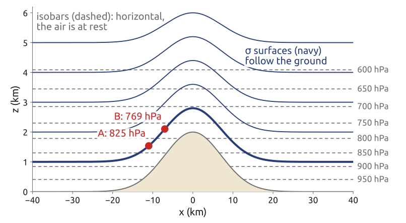
The horizontal pressure gradient at constant height, written with derivatives along a \(\sigma\) surface, follows from the chain rule. Along a \(\sigma\) surface the pressure changes both because the position changes horizontally and because the height of the surface changes: \(\nabla_\sigma p = \nabla_z p + (\partial p/\partial z)\nabla_\sigma z\), so \[ \nabla_z p = \nabla_\sigma p - \frac{\partial p}{\partial z}\,\nabla_\sigma z , \] with \(\nabla_z\) and \(\nabla_\sigma\) the horizontal gradients at constant \(z\) and at constant \(\sigma\). Over a sloping surface the two terms are large and nearly cancel; their discretization errors do not cancel, and a fluid at rest starts to move (Haney 1991). Figure 17 gives the orders of magnitude: an isothermal atmosphere at rest, with scale height 8 km, over a mountain 2 km high with a largest slope of about 1:6. Between two points A and B 4 km apart on the same \(\sigma\) surface, each term is about 14 hPa/km, while the true difference is zero. A weather pressure gradient is 1 hPa per 100 km, 0.01 hPa/km: an error of a tenth of a percent in either term is as large as the weather. The simplest discretization of the two terms between A and B (end points for the first term, the mid-point pressure for the second) leaves 0.003 hPa/km, a third of a weather gradient, in air at rest. The error grows with the slope and the stratification.
22 Schär’s mountain, and research at Polimi
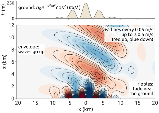
The test of Schär et al. (2002) puts these choices under strain (Figure 18): a mountain whose profile is a smooth envelope of half-width \(a = 5\) km and peak height \(h_0 = 250\) m, carrying ripples of wavelength \(\lambda = 4\) km, in a wind of 10 m/s with \(N = 0.01\) s\(^{-1}\). The ripples are narrower than \(2\pi U/N\), so their disturbance must fade with height; the envelope is wider, so it must send hydrostatic waves up. A terrain-following coordinate carries the ripples up into the domain, where its pressure-gradient errors pollute the waves; Schär et al. introduced the SLEVE (smooth level vertical) coordinate, whose surfaces lose the small scales of the terrain quickly with height. Other answers keep the coordinate surfaces flat and let the ground cut the cells (cut cells; Shaw and Weller (2016) compare them with terrain-following grids), or refine the mesh locally near the mountains. At MOX, Politecnico di Milano, Orlando et al. (2024) do the latter with an implicit–explicit discontinuous Galerkin method on non-conforming meshes, refined near the orography, and validate it on Schär’s test and on realistic profiles.
23 The tests every new dynamical core must pass
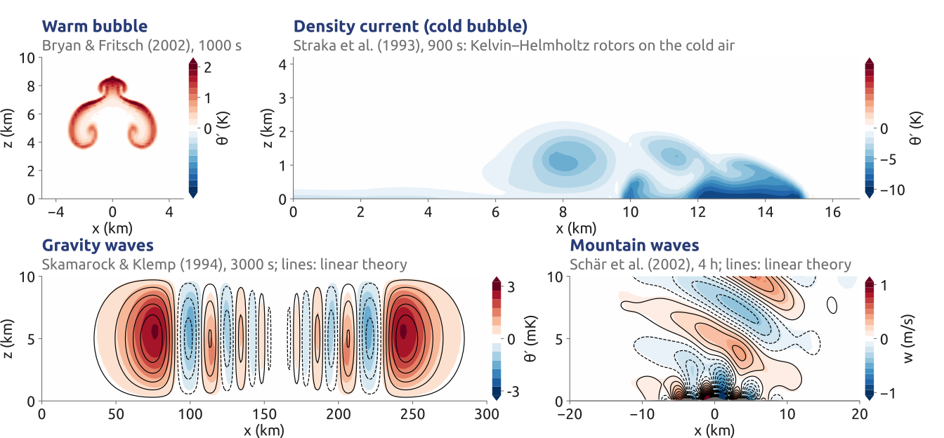
New dynamical cores are tested on a small set of vertical slices, each with a purpose (Figure 19). A rising warm bubble (Bryan and Fritsch 2002) tests nonlinear advection and buoyancy: it rises and rolls up into a mushroom. Straka’s density current, a cold bubble that falls and spreads along the ground with Kelvin–Helmholtz rotors on its top, tests a strongly nonlinear flow against a converged reference (Straka et al. 1993). The inertia–gravity waves of Skamarock and Klemp (1994), a small, smooth warm anomaly in a stratified channel with a mean wind of 20 m/s, test the linear waves against an analytic solution: here the largest \(\theta'\) is 2.80 mK against 2.73 mK in linear theory. Schär’s mountain tests the terrain (Schär et al. 2002): the largest \(w\) is 0.90 m/s against 0.89 m/s. The four runs of the figure use Gusto, a compressible Euler core built on compatible finite elements, with cells of 200 m to 2 km.
24 A compressible core on Straka’s test
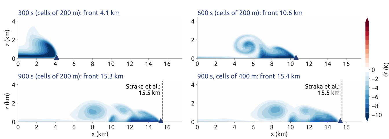
Gusto solves the compressible Euler equations for the velocity, the density and the potential temperature on an extruded mesh: the velocity in an \(H(\mathrm{div})\) space (its normal components continuous across the cell faces), the density discontinuous, and \(\theta\) in the space of the vertical velocity’s degrees of freedom, that is with \(w\) (Charney–Phillips). Its time step is semi-implicit: explicit upwind transport, and the sound and gravity waves implicit, with one elliptic problem for the pressure per iteration (Melvin et al. 2019; Natale et al. 2016). On Straka’s test with cells of 200 m, its front at 900 s (the \(-1\) K point on the ground) is at 15.3 km, 1.4% behind the reference of Straka et al. (1993) (15.54 km); a Boussinesq slice model with the same viscosity puts it at 16.8 km, 8% ahead (Figure 20). The equations matter: with the right equations and a converged reference, a model can be checked to the per cent.
25 DCMIP: eleven cores, one set of tests
The Dynamical Core Model Intercomparison Project held workshops in 2008, 2012 and 2016; the last was a two-week summer school at NCAR in June 2016, where eleven non-hydrostatic cores ran the same tests: a moist baroclinic wave, a tropical cyclone, and a supercell that splits, on a small planet (Ullrich et al. 2017, Tables 2–5). The baroclinic wave descends from the classic test of Jablonowski and Williamson (2006). The cores differ in every choice:
| Model (centre) | Grid | Horizontal | Staggering | Vertical | Time |
|---|---|---|---|---|---|
| ACME-A (Sandia, Colorado) | cubed sphere | spectral elements | A | Lorenz, floating mass | KGU53 Runge–Kutta |
| CSU (Colorado State) | geodesic | finite volumes | Z | Lorenz, height | Adams–Bashforth 3 |
| DYNAMICO (IPSL) | geodesic | finite volumes | C | Lorenz, floating mass | ARK(2,3,2) IMEX |
| FV3 (GFDL) | cubed sphere | finite volumes | D | co-located, floating mass | forward–backward, semi-implicit |
| FVM (ECMWF) | octahedral | finite volumes | A | co-located, height | semi-implicit |
| GEM (ECCC) | Yin–Yang | finite differences | C | Charney–Phillips, log pressure | semi-implicit |
| ICON (MPI-M, DWD) | icosahedral triangles | finite volumes | C | Lorenz, height | predictor–corrector |
| MPAS (NCAR) | Voronoi | finite volumes | C | Lorenz, height | split-explicit |
| NICAM (Japan) | geodesic | finite volumes | A | Lorenz, height | split-explicit |
| OLAM (Duke, Miami) | geodesic | finite volumes | C | Lorenz, height, cut cells | Adams–Bashforth 2 |
| Tempest (UC Davis) | cubed sphere | spectral elements | A | Lorenz, height | ARS(2,3,2) IMEX |
Staggering: Arakawa’s A, C and D grids; Z: vorticity, divergence and mass at the same points. Floating mass: Lagrangian vertical layers that move with the flow and are remapped. IMEX: implicit–explicit Runge–Kutta schemes (ARK, ARS). FVM is ECMWF’s finite-volume research core; the operational IFS and LFRic are not in the table. Very different formulations, judged on the same tests.
26 Four dynamical cores of today
| MPAS, MONAN | FV3 | ICON | LFRic | |
|---|---|---|---|---|
| Centre | NCAR; INPE (Brazil) | GFDL; NOAA’s GFS since 2019 | DWD, MPI-M | Met Office |
| Equations | compressible, non-hydrostatic | compressible, non-hydrostatic | compressible, non-hydrostatic | compressible, non-hydrostatic |
| Grid | Voronoi hexagons | cubed sphere | icosahedral triangles | cubed sphere |
| Space | finite volumes, C grid (TRiSK) | finite volumes, D grid | finite volumes, C grid | mixed finite elements |
| Time | split-explicit | forward–backward, implicit vertical | predictor–corrector | iterated semi-implicit semi-Lagrangian |
| Vertical | height, Lorenz | floating Lagrangian layers | height, Lorenz | height, Charney–Phillips |
The four solve the same compressible, non-hydrostatic equations with four discretizations. MPAS uses centroidal Voronoi grids, which can be refined smoothly over a region without nesting, and the C-grid scheme TRiSK of Thuburn, Ringler, Skamarock and Klemp (Skamarock et al. 2012); Brazil’s community model MONAN is built on it. FV3 runs on the cubed sphere with a D grid and vertical layers that float with the flow and are remapped, and can nest a regional grid inside the global one (Harris and Lin 2013). ICON uses icosahedral triangles with a C grid (Zängl et al. 2014). LFRic, named after Lewis Fry Richardson, uses mixed finite elements on the cubed sphere with the Charney–Phillips placement and an iterated semi-implicit semi-Lagrangian step (Melvin et al. 2019; Adams et al. 2019). Every method of the course is in a model of today (Ullrich et al. 2017).
27 Dynamical cores in the BRICS countries
| Country | Model (centre) | Grid | Method |
|---|---|---|---|
| Brazil | MONAN (INPE), MPAS-based | Voronoi | finite volumes (TRiSK) |
| Brazil | BAM (CPTEC/INPE) | Gaussian | spectral, semi-implicit, Eulerian or SL |
| Russia | SL-AV (Hydrometcentre) | reduced lat–lon | finite differences, SISL |
| India | HGFM / BFS (IITM) | cubic octahedral | spectral, SISL |
| India | NCUM (NCMRWF; the Met Office’s UM) | lat–lon, C grid | finite differences, SISL |
| China | GRAPES / CMA-GFS (CMA) | lat–lon | finite differences, SISL |
| China | YHGSM (NUDT) | Gaussian | spectral, SISL |
| South Africa | UM (SAWS; Met Office) | lat–lon, C grid | finite differences, SISL |
SISL: semi-implicit semi-Lagrangian; SL: semi-Lagrangian; lat–lon: latitude–longitude. The operational global models of the BRICS countries are spectral (BAM in Brazil (Figueroa et al. 2016), HGFM in India (Krishna et al. 2025), YHGSM in China (Jiang et al. 2021)) or grid-point latitude–longitude models (SL-AV in Russia (Tolstykh et al. 2017), GRAPES/CMA-GFS in China, and the Met Office’s Unified Model (Brown et al. 2012) in India and South Africa), nearly all with semi-implicit semi-Lagrangian steps; Brazil’s new community model MONAN is built on MPAS (Skamarock et al. 2012). The entry for GRAPES/CMA-GFS follows Pedro Peixoto’s BRICS 2026 talk. SISL steps, on many grids, are the workhorse of operational centres.
28 What a weather app shows: four global models
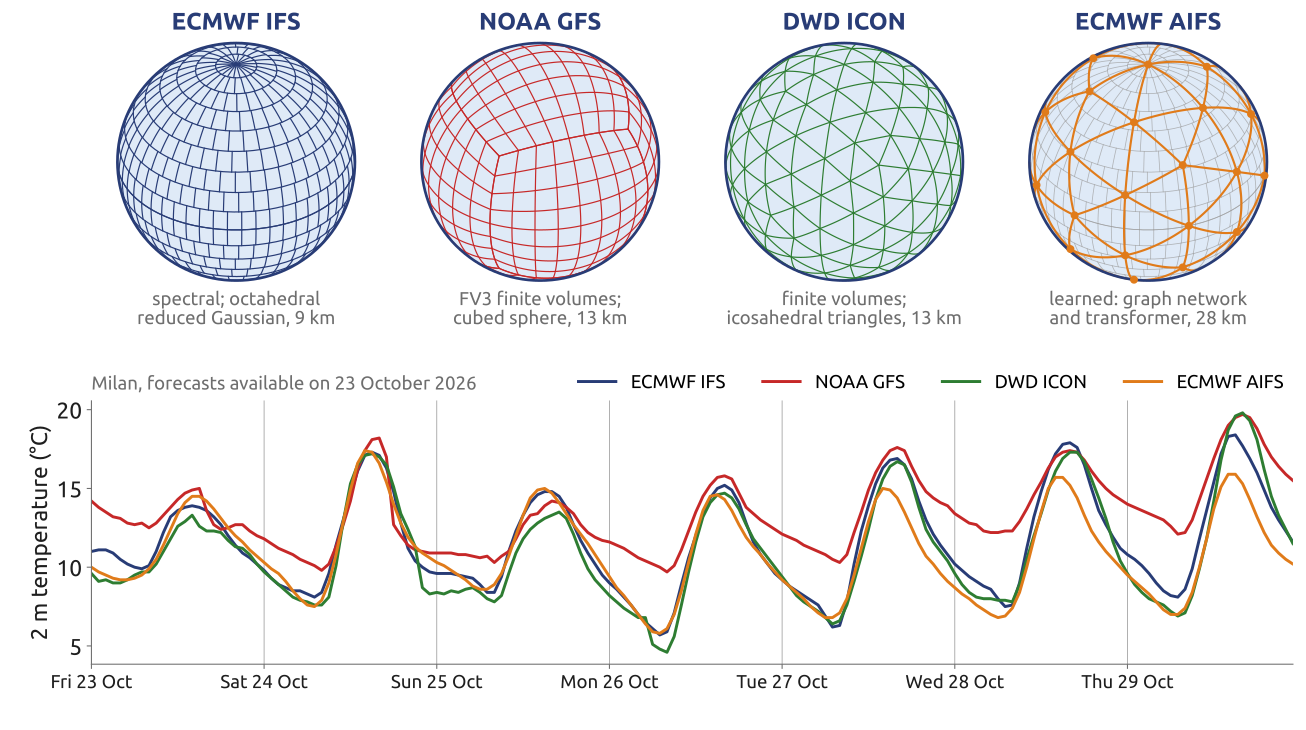
Weather apps such as Windy.com show several global models side by side: ECMWF’s IFS (spectral, on an octahedral reduced Gaussian grid, 9 km), NOAA’s GFS (the FV3 finite-volume core on a cubed sphere, 13 km), DWD’s ICON (finite volumes on icosahedral triangles, 13 km) and ECMWF’s AIFS (a learned model, a graph network with a transformer, on a reduced Gaussian grid of about 28 km). For Milan their forecasts of the 2 m temperature, made from the runs available on 23 October 2026, differ by degrees (Figure 21). The forecast read on a phone is one model among several, each with its own numerics; the spread among them, as among the members of an ensemble, is a measure of the uncertainty.
29 Ocean models (1/3): the first one, 1969
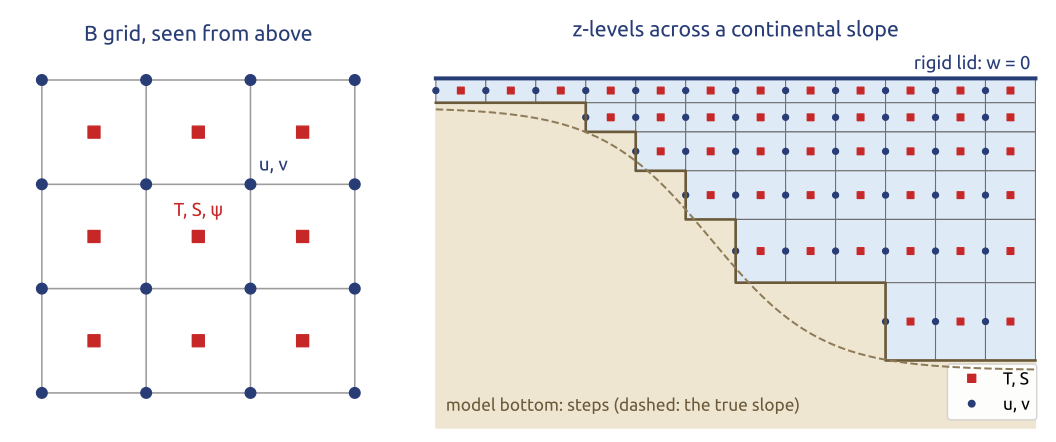
Kirk Bryan’s model at GFDL (Bryan 1969) was the first general circulation model of the world ocean, with coasts and bottom topography. It solves the hydrostatic, Boussinesq primitive equations, \[ \frac{D\mathbf u}{Dt} + f\,\mathbf k\times\mathbf u = -\frac{1}{\rho_0}\nabla\,\delta p + \mathbf F, \qquad \frac{\partial\,\delta p}{\partial z} = \rho_0 b, \qquad \nabla\cdot\mathbf u + \frac{\partial w}{\partial z} = 0, \] \[ \frac{DT}{Dt} = Q_T, \qquad \frac{DS}{Dt} = Q_S, \qquad b = b(T, S, z), \qquad w|_{z=0} = 0 \ \text{(rigid lid)}, \] with \(\mathbf u = (u, v)\) the horizontal and \(w\) the vertical velocity, \(\mathbf k\) the vertical unit vector, \(\rho_0\) a reference density, \(\delta p\) the departure of the pressure from a reference profile, \(b\) the buoyancy, \(T\) and \(S\) temperature and salinity, and \(\mathbf F\), \(Q_T\), \(Q_S\) the eddy mixing. The grid has fixed depths (\(z\)-levels), the bottom drawn in steps, and Arakawa’s B grid in the horizontal: \(T\), \(S\) and the transport streamfunction \(\psi\) at the centres of the cells, both velocity components at the corners (Figure 22). The rigid lid \(w = 0\) at the surface removes the fast surface gravity waves, about 200 m/s in a 4 km ocean, which would force steps of minutes; the price is that the depth-integrated flow comes from a streamfunction \(\psi\), through an elliptic problem at every step, as in the 1950 forecast. With it, Manabe and Bryan (1969) coupled ocean and atmosphere for the first time, and the code of Bryan, Cox and Semtner became GFDL’s Modular Ocean Model, MOM (Griffies et al. 2000).
30 Ocean models (2/3): the vertical coordinate
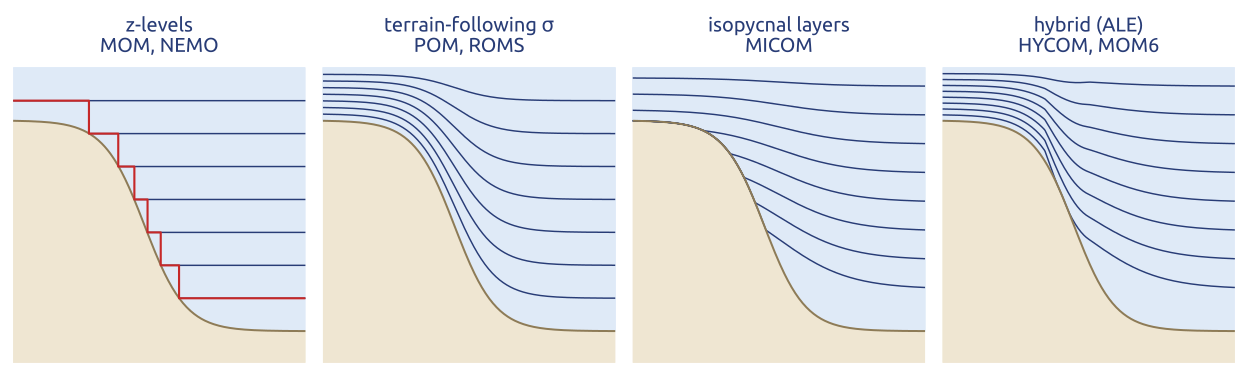
For thirty years ocean modellers debated one choice: how the layers of the model follow the ocean (Figure 23; Griffies et al. (2000)).
- \(z\)-levels (MOM, OPA/NEMO): simple, with an exact horizontal pressure gradient; the bottom is a staircase, eased by partial steps.
- Terrain-following \(\sigma\) (POM (Blumberg and Mellor 1987), ROMS (Shchepetkin and McWilliams 2005)): smooth over shelves and slopes, the coordinate for coasts; but the same pressure-gradient error as in the atmosphere over steep slopes (Haney 1991).
- Isopycnal (MICOM): the layers are density surfaces. The interior ocean mixes mostly along them, and \(z\)-level advection adds spurious mixing across them; isopycnal layers have none, but they vanish where they outcrop.
- Hybrid and ALE (arbitrary Lagrangian–Eulerian; HYCOM (Bleck 2002), MOM6): \(z\) near the surface, isopycnal in the interior, \(\sigma\) on the shelf, with layers that move and are remapped.
A free surface replaced the rigid lid: the fast, depth-integrated (barotropic) mode is stepped separately with short steps, a split-explicit scheme, as in POM and ROMS (Shchepetkin and McWilliams 2005).
31 Ocean models (3/3): the grids of today
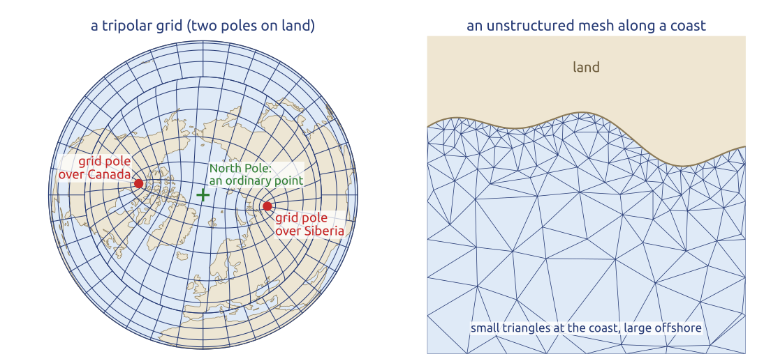
The ocean has only one pole problem: the South Pole is on land, the North Pole in the Arctic Ocean. Tripolar grids (Murray 1996) keep a latitude–longitude grid south of the Arctic and, in the Arctic, a grid with two poles placed on land, over Canada and Siberia, so that no grid pole lies in the ocean (Figure 24): NEMO’s ORCA grids (Madec et al. 2026) and GFDL’s MOM. MOM6 (Adcroft et al. 2019) uses a C grid and a vertical Lagrangian-remap (ALE) coordinate, at \(1/4^\circ\) and \(1/2^\circ\). Unstructured meshes put small cells along coasts and straits and large ones elsewhere: FESOM2 with finite volumes on triangles (Danilov et al. 2017), MPAS-Ocean on Voronoi cells (Ringler et al. 2013), ICON-O on a triangular C grid (Korn 2017). How fine? Hurlburt and Hogan (2000) simulated the Gulf Stream at \(1/8^\circ\) to \(1/64^\circ\).
32 The ocean’s eddies set the grid
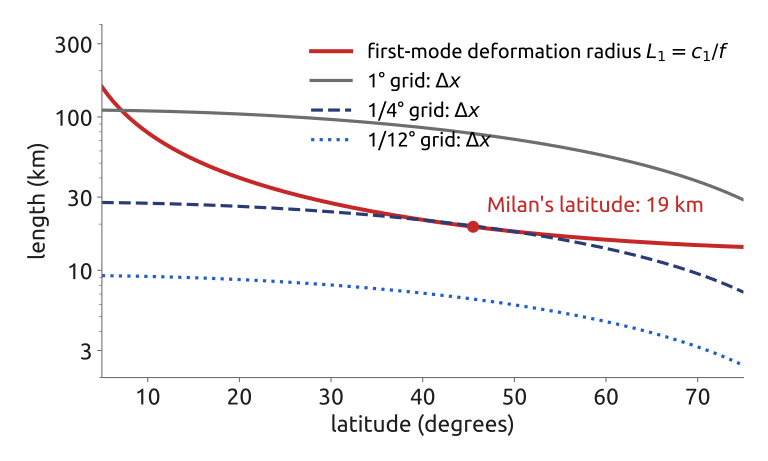
The ocean’s weather, its mesoscale eddies, has the size of the first baroclinic deformation radius \[ L_1 = \frac{c_1}{f}, \] with \(c_1\) the speed of the first baroclinic mode and \(f\) the Coriolis parameter. With \(c_1 \approx 2\) m/s, \(L_1\) is about 20 km at the latitude of Milan, against about 1000 km for the atmosphere’s cyclones (the deformation radius \(L_d = NH/f\) of Vallis (2017) is \(\pi\) times larger than \(L_1\)). A grid resolves these eddies only where the grid spacing \(\Delta x\) is smaller than \(L_1\): at \(45^\circ\)N a \(1/4^\circ\) ocean grid has about one cell per \(L_1\), too coarse, and a \(1/12^\circ\) grid about three (Figure 25). The ratio \(L_1/\Delta x\) decides (Cushman-Roisin and Beckers 2011). The ocean’s weather is ten times smaller than the atmosphere’s, so ocean models need grids ten times finer.
33 Key points
- 1950 to the 1960s: from one equation to the primitive equations and general circulation models; Lorenz: chaos, hence ensembles.
- Finite differences on latitude–longitude grids: the polar cells set the time step; semi-implicit semi-Lagrangian steps.
- Spectral transforms: no pole problem, easy semi-implicit solves; but \(N^3\) transforms and global communication: the scalability problem.
- Quasi-uniform grids: cubed sphere, icosahedral, Voronoi; local finite volumes and elements.
- The vertical: Charney–Phillips staggering; an implicit vertical for sound; a sponge at the top; terrain-following coordinates and their pressure-gradient error.
- Tests: bubbles, density currents, mountains; DCMIP: very different cores, the same tests.
- Ocean: rigid lid to free surface; \(z\), \(\sigma\), isopycnal and ALE; tripolar and unstructured grids; eddies need \(1/10^\circ\).
Today’s models assemble the same methods, each in its own way.
Further reading
Williamson (2007) for the history of dynamical cores; Staniforth and Thuburn (2012) for the grids on the sphere; Randall et al. (2019) for a century of Earth system models; Ullrich et al. (2017) for the design of today’s non-hydrostatic cores; Griffies et al. (2000) for ocean models; Durran (2010), Ch. 7, for semi-Lagrangian methods; Kalnay (2003) for predictability and ensembles; Bauer et al. (2021) for the computing challenge.