November 2026 · Politecnico di Milano

Modern weather, ocean and climate models

Atmosphere and Ocean Dynamics — Lecture 9

Prof. Dr. Pedro da Silva Peixoto

Applied Mathematics
Instituto de Matemática e Estatística
Universidade de São Paulo

Visiting Professor at MOX Lab
Politecnico di Milano

Warm-up

1. What equations are used in global weather forecasting?
2. What equations are used in global ocean modelling?
3. What methods are used to discretize the equations?

The whole course, from memory: answer on paper first, 3 minutes. Today: how the models of today got there, from 1950 onwards.

Answers: (1) the compressible, non-hydrostatic Euler equations (ICON, MPAS, FV3, LFRic, the UM) or the hydrostatic primitive equations (the IFS, BAM), with moisture and parameterized physics. (2) The hydrostatic, Boussinesq primitive equations with a free surface (NEMO, MOM6, FESOM, MPAS-Ocean). (3) Finite differences and finite volumes (on latitude–longitude or quasi-uniform grids), spectral transforms (the IFS), finite and spectral elements (LFRic, CAM-SE); in time, semi-implicit semi-Lagrangian, split-explicit or Runge–Kutta steps.

Where we are and where we are going

Previous knowledge

• Weather: the compressible, non-hydrostatic Euler equations, or the hydrostatic primitive equations, with moisture and parameterized physics
• Ocean: the hydrostatic, Boussinesq primitive equations, with a free surface
• Methods: finite differences and volumes, spectral transforms, finite elements; the CFL condition; semi-implicit and semi-Lagrangian steps
• The 1950 forecast; the vertical slice and its tests

Where we are going

1. From 1950 to the 1960s
2. Finite differences and the pole problem
3. Spectral models and the scalability problem
4. Quasi-uniform grids; notebook
5. The vertical
6. Tests, DCMIP, the models of today
7. Ocean models since 1969

How the models of today assemble the methods of this course, and how they got there

(Williamson 2007; Staniforth and Thuburn 2012; Randall et al. 2019)

Two minutes. Left: what we take as known (the whole course; the warm-up checked it). Right: the road of the day, the history from lecture 1 continued from 1950; each item links to its first slide.

1950: one equation, one layer

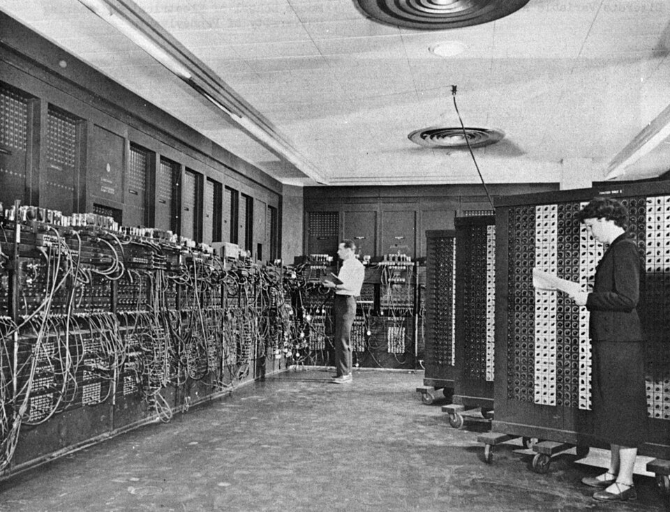
The ENIAC at Aberdeen. U.S. Army photo, public domain

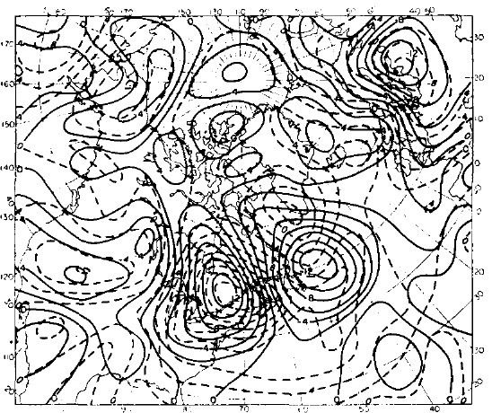
24-h change of 500 hPa height, 30 Jan. 1949: observed (solid), computed (dashed). CC BY 4.0

\[\frac{\partial\zeta}{\partial t} + J(\psi, \zeta + f) = 0, \qquad \nabla^2\psi = \zeta\]

\(\zeta\): vorticity; \(\psi\): streamfunction; \(J(\psi, q)\): advection of \(q\); \(f\): Coriolis parameter

• Charney, Fjørtoft and von Neumann: finite differences on a 736 km grid, 3-hour steps; 24 hours of computing for a 24-hour forecast
• No gravity waves, so the initial state needed no balancing

But: one level of one variable. How do we get the whole atmosphere?

The first forecast by numbers that worked: one equation, one layer, a Poisson problem at every step

(Charney et al. 1950; Lynch 2008) · Photo: commons.wikimedia.org: ENIAC · Map: doi:10.3402/tellusa.v2i4.8607, Fig. 3c

Recall of lecture 1. Ask first: what did the 1950 model leave out that a weather model needs? (The vertical, temperature, moisture, gravity waves, the whole globe.)

1950–1975: towards the general circulation

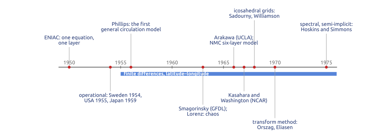
• Operational barotropic forecasts: Sweden 1954, the USA 1955, Japan 1959
• Phillips (1956): two levels, a month of the general circulation: the first climate model

• The 1960s: the primitive equations come back, with better initial states: GFDL, UCLA, NCAR; at NMC operational from 1966
• All on latitude–longitude grids, with finite differences

In twenty years, from one equation for one layer to general circulation models

(Phillips 1956; SMAGORINSKY 1963; KASAHARA and WASHINGTON 1967; Shuman and Hovermale 1968; Randall et al. 2019)

Smagorinsky (1963): the GFDL primitive-equation model; Mintz and Arakawa at UCLA (Arakawa’s Jacobian, 1966, and his staggered grids); Kasahara and Washington (1967) at NCAR; Shuman and Hovermale (1968): the NMC six-layer model, operational from 1966. Climate modelling starts: Manabe and Bryan (1969) couple the ocean (lecture 1).

1963: Lorenz and the limits of prediction

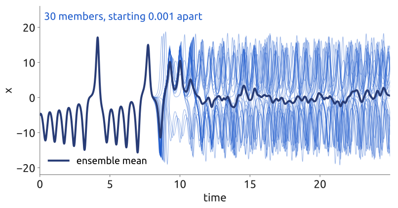
• Lorenz (1963): in a chaotic system, tiny differences grow until two forecasts are unrelated
• The limit of predictability of the weather: about two weeks
• Hence ensembles: many forecasts from slightly different states; their spread says how much to trust them

But: each member is a full model. On which grid?

A single forecast is not enough: predict the uncertainty too

(Lorenz 1963; Kalnay 2003)

Ask first: two forecasts differ by 0.001 at the start: when do they disagree completely? ECMWF’s ensemble: 50 perturbed members and a control.

Finite differences and the pole problem

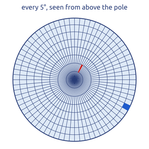
• 1960s–1980s: finite differences on latitude–longitude grids, as Richardson’s: GFDL, UCLA (Arakawa’s staggered grids), NCAR, NMC
• The meridians meet at the poles: the cells become thin wedges
• The CFL condition forces tiny time steps there; fixes: polar filters, fewer points near the poles

But: how small is “tiny”?

On a latitude–longitude grid, the cells at the poles set the time step of the whole model

(Staniforth and Thuburn 2012; Williamson 2007)

CFL: lecture 5. Ask first: a 0.25-degree grid: what is the east-west spacing in the last row? Old fixes: filters at high latitudes, reduced grids (fewer points near the poles).

In class: the pole problem in numbers

Exercise 1 — The pole problem. A latitude–longitude grid with a spacing of \(0.25^\circ\) (\(1440\times720\) points). Compute the east–west spacing \(\Delta x = a\cos\varphi\,\Delta\lambda\) at the equator, at \(60^\circ\)N and in the last row, \(89.875^\circ\)N, and the largest stable explicit time step \(\Delta t = \Delta x/c\) for gravity waves with \(c = 300\) m/s.

	equator	\(60^\circ\)N	\(89.875^\circ\)N
\(\Delta x\)
\(\Delta t = \Delta x / c\)

\(a = 6371\) km, \(\;\Delta\lambda = 0.25^\circ = 4.36\times10^{-3}\) rad.

To hand in. A quasi-uniform grid with the same number of columns: its mean spacing \(\sqrt{4\pi a^2/N}\) and its time step. How many columns does a global grid of 1 km need?

In notebook 09a (❗ 6.1): open in Colab · download

(Staniforth and Thuburn 2012)

Answers: 27.8 km, 13.9 km, 61 m; 93 s, 46 s, 0.2 s. Hand-in: N = 1.04e6, spacing 22 km, 74 s; 1 km: 5.1e8 columns.

What the exercise showed

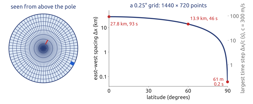
• \(\Delta x\): 27.8 km at the equator, 13.9 km at \(60^\circ\)N, 61 m in the last row; \(\Delta t\): 93 s, 46 s, 0.2 s

• A quasi-uniform grid with the same \(1.04\times10^6\) columns: mean spacing 22 km, \(\Delta t = 74\) s; a global 1 km grid needs \(5.1\times10^8\) columns

The last row near the pole sets the time step of the whole latitude–longitude model

(Staniforth and Thuburn 2012; Williamson 2007)

Old fixes: filters at high latitudes, reduced grids (fewer points near the poles), and long steps (semi-implicit semi-Lagrangian, next).

Semi-Lagrangian: follow the air back

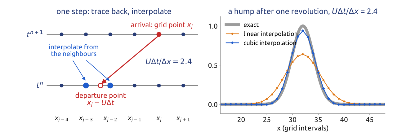
• The value arriving at \(x_j\) is the value at the departure point \(x_j - U\Delta t\), interpolated
• Stable for any Courant number \(U\Delta t/\Delta x\): the stencil moves with the departure point

• With semi-implicit gravity waves: steps of minutes at 9 km (SISL; Robert 1981)
• Linear interpolation damps; mass is not conserved exactly

\(x_j\): grid point \(j\); \(\Delta x\): grid spacing; \(U\): wind speed; \(\Delta t\): time step

CFL still holds: the trajectory puts the true domain of dependence inside the stencil

(Durran 2010, Sect. 7.1; Staniforth 1997)

Semi-implicit: lecture 7. Ask first: Courant number 2.4 with an explicit Eulerian scheme? (Unstable: the information comes from outside the stencil.) Linear interpolation = upwind on a shifted stencil, damping as |A|² = 1 − 2α(1−α)(1 − cos kΔx), α the fractional part of the Courant number (Durran 7.1.1). Models use cubic interpolation; conserving variants exist (e.g. ENDGame’s mass fix).

The spectral era (1970s–today)

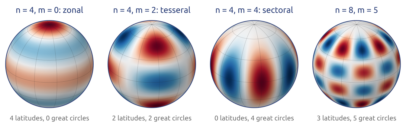
• Transform method (Orszag 1970; Eliasen et al. 1970): derivatives exact in spectral space, products on the grid: no pole problem
• Multi-level, semi-implicit (Bourke 1974; Hoskins and Simmons 1975): the Helmholtz problem of the gravity waves is diagonal in spherical harmonics
• ECMWF: spectral from 1983, semi-Lagrangian from 1991: steps of many minutes
• For forty years the method of most global forecasts

Spectral transforms removed the pole problem and made semi-implicit steps easy

(Orszag 1970; Eliasen et al. 1970; Bourke 1974; HOSKINS and SIMMONS 1975; Simmons et al. 1989; Ritchie et al. 1995)

Spherical harmonics, the transform method and the semi-implicit solve: lecture 7. ECMWF’s first operational forecast (1979) was a grid-point model; its spectral model followed in 1983 (Simmons et al. 1989).

Spectral models today

Model (centre)	Resolution	Levels	Time step
IFS (ECMWF, Europe)	about 9 km (TCo1279)	137	SISL
YHGSM (NUDT, China)	about 15 km (TL1279)	137	SISL
HGFM / BFS (IITM, India)	about 6.5 km (TCo1534)	64	SISL
BAM (CPTEC/INPE, Brazil)	about 20 km	96	semi-implicit, Eulerian or SL
GSM (JMA, Japan)	about 13 km (TQ959)	128	SISL
ARPEGE (Météo-France), stretched	about 7 km over France (T1198)	105	SISL
GFS (NOAA, USA), 1980–2019	about 13 km (TL1534)	64	SISL
AROME (Météo-France), limited area	1.3 km (bi-Fourier)	90	SISL
EC-Earth3 (Europe), climate	about 80 km (TL255)	91	SISL

“The state of the art of the millennium”: pseudo-spectral, semi-implicit, semi-Lagrangian

(Krishna et al. 2025; Figueroa et al. 2016; Japan Meteorological Agency 2024; Météo-France 2016; Döscher et al. 2022; Staniforth and Thuburn 2012)

SISL: semi-implicit semi-Lagrangian. TCo: cubic truncation on an octahedral grid; TQ: quadratic; TL: linear. ARPEGE: stretched (Schmidt), 7 km over France to 33 km over the South Pacific (2016 report); AROME: Fourier in x and y. IFS, YHGSM, HGFM, BAM and GFS after Pedro’s BRICS 2026 talk (table “The state-of-the-art of the millennium”).

The scalability problem

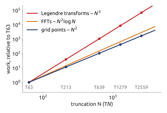
• A forecast must finish in about an hour, on machines of \(10^5\)–\(10^6\) cores
• Halve the spacing (double the truncation \(N\)): 4 times the grid points, 8 times the Legendre transforms
• Every transform needs data from the whole globe: global communication; so do the large linear solves of semi-implicit grid-point models
• “Fast” Legendre transforms delay it (Wedi et al. 2013); local methods avoid it

Spectral models do not scale on today’s computers: the reason for a new generation of models

(Williamson 2007; Wedi et al. 2013; Bauer et al. 2021)

Figure: lecture 7 (operation counts, Williamson 2007). Pedro’s talks: CPTEC’s TUPÃ (about 30 000 cores, 2013) could not finish high-resolution spectral forecasts in the time window.

The kilometre scale

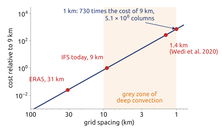
• Halve the grid spacing \(\Delta x\): 4 times the columns, half the time step (CFL): 8 times the cost
• At a few km, deep convection starts to be resolved: the “grey zone” of the parameterizations
• 1.4 km global IFS, a four-month simulation (Wedi et al. 2020)
• Codes reach about 5% of peak speed: memory and communication, not arithmetic, limit them; hence GPUs and local stencils

The kilometre scale costs about a thousand times today’s forecast: methods must scale

(Wedi et al. 2020; Bauer et al. 2021; Adams et al. 2019)

Ask first: from 9 km to 1 km, how much more work? ((9)³ ≈ 730, more with more levels.) Global transforms against local stencils: lectures 7–8. LFRic (GungHo) was designed for scalability: no global transforms, a cubed sphere without poles.

Three answers to the pole problem

1. Spectral transforms

Spherical harmonics have no pole problem: ECMWF’s IFS. The Legendre transforms grow costly at high resolution

2. Long time steps

Semi-implicit (fast waves implicit) and semi-Lagrangian (follow the flow back): steps much longer than an explicit Eulerian scheme allows (IFS, the Met Office’s ENDGame)

3. Quasi-uniform grids

Cells of nearly the same size everywhere: cubed sphere, icosahedral triangles, Voronoi hexagons

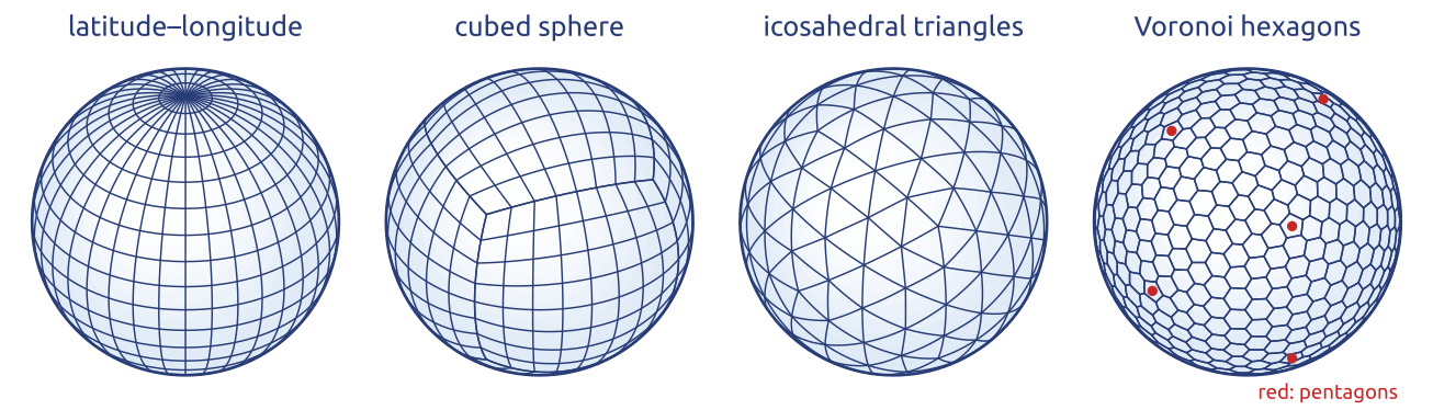
Change the basis, the time step, or the grid

(Staniforth and Thuburn 2012; Williamson 2007)

A recap of the last slides. Spherical harmonics, semi-implicit steps: lecture 7. Semi-Lagrangian: the step is no longer limited by the Eulerian CFL condition (the departure point carries the domain of dependence). Semi-implicit: the gravity-wave terms implicit (a Helmholtz problem every step).

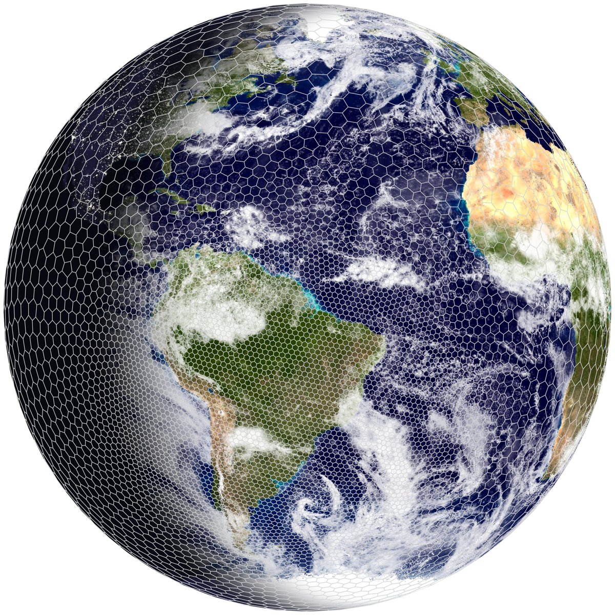
The new generation: quasi-uniform grids

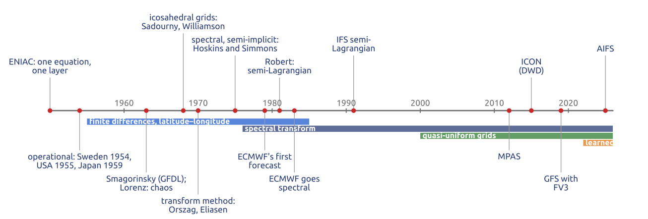
• An old idea: icosahedral grids in 1968 (Sadourny, Arakawa and Mintz; Williamson), not competitive then
• Since about 2000: cubed sphere (FV3, LFRic), icosahedral triangles (ICON), Voronoi (MPAS, MONAN)

• Local methods: finite volumes and finite elements, communication only with neighbours
• But: no grid on the sphere is perfect. What does each model choose?

Quasi-uniform grids and local operators: models built to scale

(SADOURNY et al. 1968; WILLIAMSON 1968; Staniforth and Thuburn 2012)

Sadourny (1972) also tried the cubed sphere. Pedro’s talks: “not competitive with latitude-longitude grids at the time”. Finite volumes: lecture 6; finite elements: lecture 8.

Notebook Grids on the sphere

Notebook 09a (open in Colab · download): build a grid like MONAN’s in a few lines of Python.

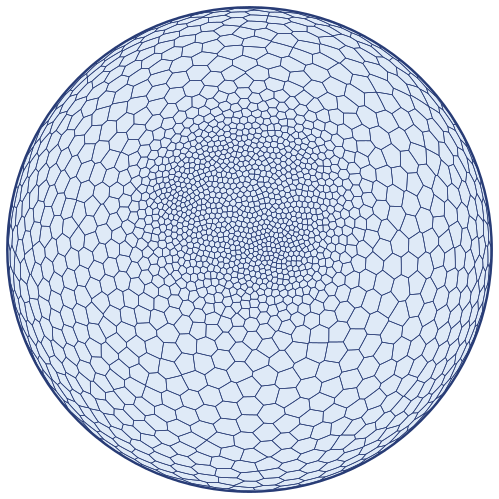
A Voronoi grid refined over the Alps

1. Delaunay and Voronoi in the plane
2. On the sphere: six points make a cube
3. Icosahedral grids: hexagons and 12 pentagons
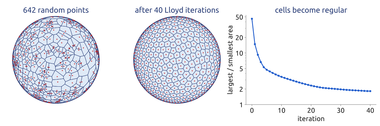
4. Lloyd’s iterations: from random points to a regular grid
5. Local refinement over the Alps ❗ 5.1
6. The time step of the smallest cell; the pole problem ❗ 6.1

Predict, run, explain: how much smaller do the cells get for a density 256 times larger?

Build a grid like MONAN’s in a few lines of Python

(Ringler et al. 2011; Staniforth and Thuburn 2012)

In class, 20 min: sections 1 to 5; 6 at home. Adapted from the 2023 MONAN course notebook. Runs in about 30 s.

What the notebook showed

• Icosahedral grids: \(10\cdot4^n+2\) cells; all hexagons except 12 pentagons
• Lloyd’s iterations: random points → a centroidal Voronoi grid

• Refinement: \(\Delta x \propto \rho^{-1/4}\) (density ×256, cells ÷4); the smallest cell sets the time step
• The same grids carry the vertical columns of the model

Quasi-uniform grids remove the pole problem; refinement puts the small cells where we want them

(Ringler et al. 2011)

The 2.27 million cells of a 15 km grid (🧩 3.1 of the notebook): one state is 10^9 numbers.

Where the variables sit

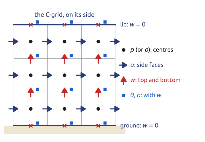
• The C grid, on its side: \(p\) at the centres, \(u\) on the side faces, \(w\) on the top and bottom faces
• \(\theta\) (or \(b\)) with \(w\): buoyancy acts on \(w\) with no averaging (Charney–Phillips)
• \(w = 0\) on the ground and the lid: imposed exactly, on the faces
• A slice model in vorticity form keeps \(\psi\), \(\xi\), \(b\) at the same points: it needs no staggering

\(u\), \(w\): horizontal and vertical velocity; \(p\): pressure; \(\theta\): potential temperature; \(b\): buoyancy; \(\psi\): streamfunction; \(\xi\): vorticity of the slice

The vertical has its own staggering choices, as the horizontal did

(Holdaway et al. 2013; Melvin et al. 2019)

C grid: lecture 6. The lowest-order compatible finite elements of Gusto and LFRic place the variables exactly so (lecture 8).

Lorenz and Charney–Phillips grids

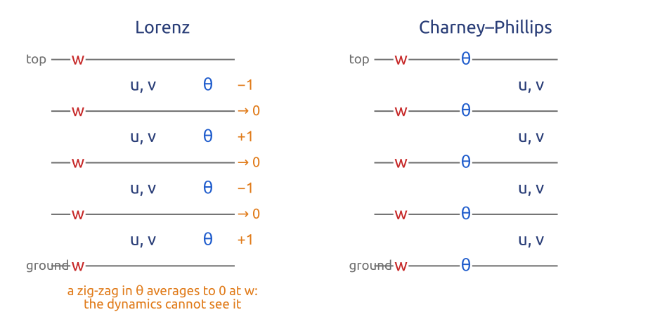
• Lorenz grid: \(\theta\) with the winds, \(w\) between: \(\theta\) must be averaged where buoyancy acts
• Charney–Phillips grid: \(\theta\) with \(w\): buoyancy where it is used
• Lorenz’s averaging hides a zig-zag in \(\theta\): a computational mode (as the A grid’s checkerboard)

\(u\), \(v\): horizontal velocity; \(w\): vertical velocity; \(\theta\): potential temperature

Staggering matters in the vertical too: Charney–Phillips for waves, Lorenz for conservation

(Holdaway et al. 2013)

A-grid checkerboard: lectures 5–6. Holdaway et al. (2013): Charney-Phillips is better for waves and PV, Lorenz for conservation (and the stable boundary layer); the Met Office uses Charney-Phillips, ECMWF a Lorenz variant. Ongoing debate.

Each step: a Poisson problem, or fast sound

• Boussinesq, anelastic: no sound waves; an elliptic (Poisson) problem gives the pressure, or the streamfunction \(\psi\), at every step, as in the 1950 forecast and the vorticity–streamfunction slice
• Compressible, non-hydrostatic (WRF, MPAS, ICON, the UM): sound waves; on the thin layers near the ground an explicit step must be tiny (right)
• HEVI (horizontally explicit, vertically implicit): the vertical sound implicit, one tridiagonal solve per column of \(J\) levels, \(O(J)\) operations
• Or semi-implicit in all directions: a Helmholtz problem each step (IFS, Gusto)

\[\Delta t \le \frac{\Delta z}{c_s} = \frac{20\ \mathrm{m}}{340\ \mathrm{m/s}} \approx 0.06\ \mathrm{s}\]

\(\Delta t\): time step; \(\Delta z\): thickness of a layer near the ground; \(c_s\): speed of sound

Somewhere there is always an elliptic or implicit solve: the price of fast waves

(Durran 2010; Klemp et al. 2007)

Split-explicit (WRF, MPAS): small steps for the acoustic modes, implicit in the vertical. IFS: lecture 7; Gusto: lecture 8.

The top of the model: let the waves out

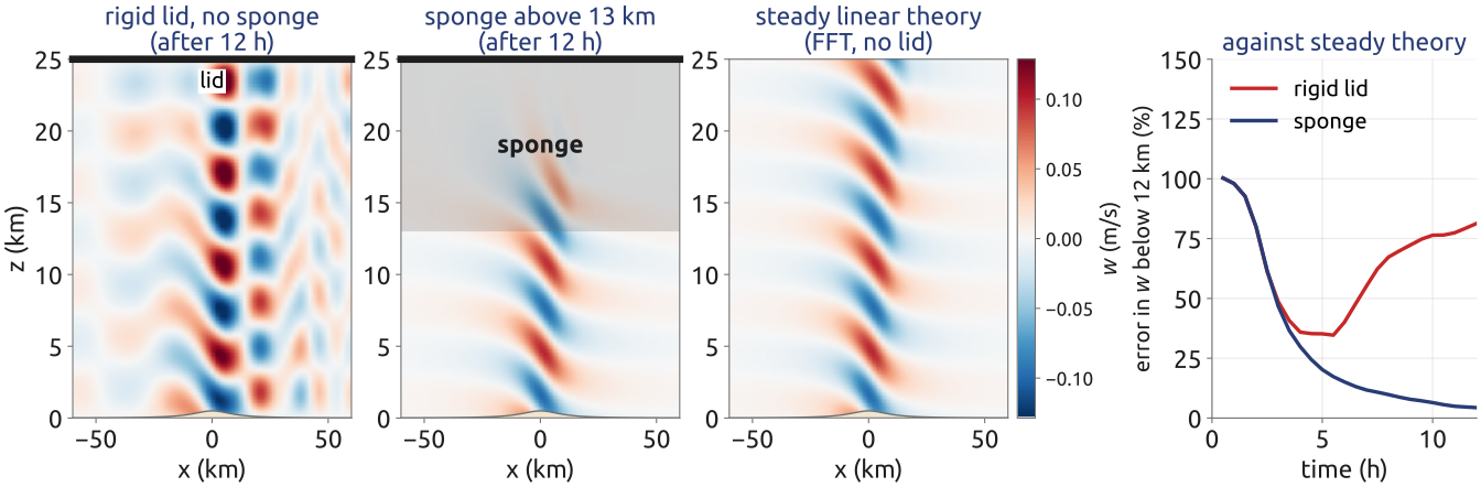
A rigid lid reflects the waves back down: a wrong, standing pattern (error 81% after 12 h). A sponge layer in the top 12 km, Rayleigh damping \(-\gamma(z)\,\xi\) and \(-\gamma(z)\,b'\), absorbs them (4%), if deep and gentle enough

\(\gamma(z)\): damping rate, zero below the sponge; \(\xi\): vorticity of the slice; \(b'\): buoyancy perturbation; \(w\): vertical velocity. A linear slice model: wind 10 m/s over a 100 m ridge (drawn 5 times higher)

A finite domain must let the waves leave: the sponge, a piece of numerics with no physics in it

(Klemp and Lilly 1978; Klemp et al. 2008)

Ask first: the model has a lid (here at 25 km); mountain waves go up: what happens? (They reflect.) Notebook 04b: error after 12 h 81 % with the lid, 4 % with a 12 km sponge; too strong or too thin also reflects.

Vertical coordinates

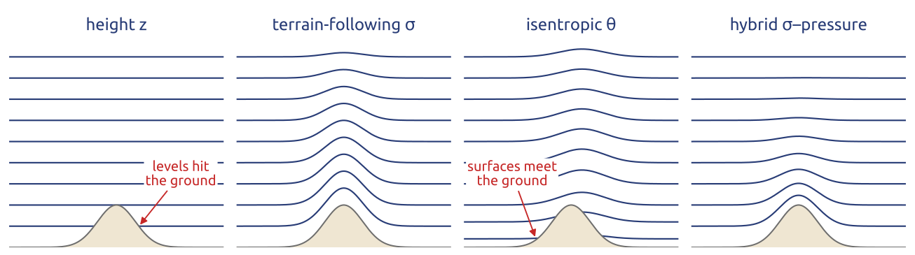
	height \(z\)	terrain-following \(\sigma\)	isentropic / isopycnal	hybrid
+	simple, exact pressure gradient	smooth over mountains	follows the flow: little false mixing	follows the ground low down, flat aloft
−	steps at the ground	error over steep slopes	surfaces meet the ground	more complex

\(z\): height; \(\sigma\): a terrain-following coordinate, constant on the ground; \(\theta\): potential temperature

No vertical coordinate is best everywhere: models mix them

(Gal-Chen and Somerville 1975; Schär et al. 2002; Griffies et al. 2000)

ECMWF: hybrid sigma-pressure (137 levels). Ocean: z-levels (NEMO), isopycnal (HYCOM in the deep), ALE (MOM6): the layers move with the flow and are remapped.

The pressure-gradient error of \(\sigma\) coordinates

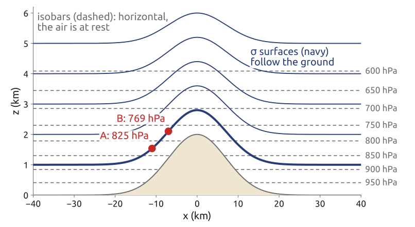
Along a sloping \(\sigma\) surface the model sees a difference of two large terms:

\[\nabla_z p = {\color{#1f5ccc}\nabla_\sigma p} - {\color{#c62828}\frac{\partial p}{\partial z}\,\nabla_\sigma z}\]

\(p\): pressure; \(z\): height; \(\nabla_z\), \(\nabla_\sigma\): horizontal gradients at constant \(z\) and at constant \(\sigma\)

• Here, from A to B: each term \(\approx 14\) hPa/km; true difference: 0 (rest)
• A weather gradient: 1 hPa per 100 km \(= 0.01\) hPa/km
• An error of 0.1% in either term is as large as the weather: a spurious wind

Following the terrain is convenient, but a small difference of large numbers is dangerous

(Haney 1991; Schär et al. 2002)

Ask first: an atmosphere (or an ocean) at rest over a mountain, sigma coordinates: will the model stay at rest? (No.) The simplest discretization of the two terms between A and B leaves 0.003 hPa/km (figure script): a third of a weather gradient, from nothing. Grows with slope and stratification.

Schär’s mountain, and research at Polimi

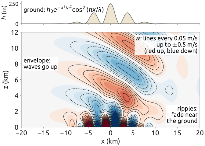
\(h_0 = 250\) m: peak height; \(a = 5\) km: envelope half-width; \(\lambda = 4\) km: ripple wavelength; \(w\): vertical velocity. Steady linear solution, wind 10 m/s

• Schär et al. (2002): a mountain with ripples. The ripples’ waves must fade; the envelope’s must go up
• A hard test for \(\sigma\) coordinates: SLEVE (smooth level vertical coordinate) flattens the coordinate surfaces aloft
• Other answers: cut cells (the ground cuts the grid cells), and local refinement with discontinuous Galerkin near the mountains (Orlando, Benacchio and Bonaventura 2024, MOX)

Mountains are still a research question for dynamical cores, here in Milan too

(Schär et al. 2002; Shaw and Weller 2016; Orlando et al. 2024)

Orlando et al. 2024 (QJRMS): IMEX-DG in deal.II, non-conforming meshes refined near the orography, validated on Schär’s test and realistic profiles.

The tests every new dynamical core must pass

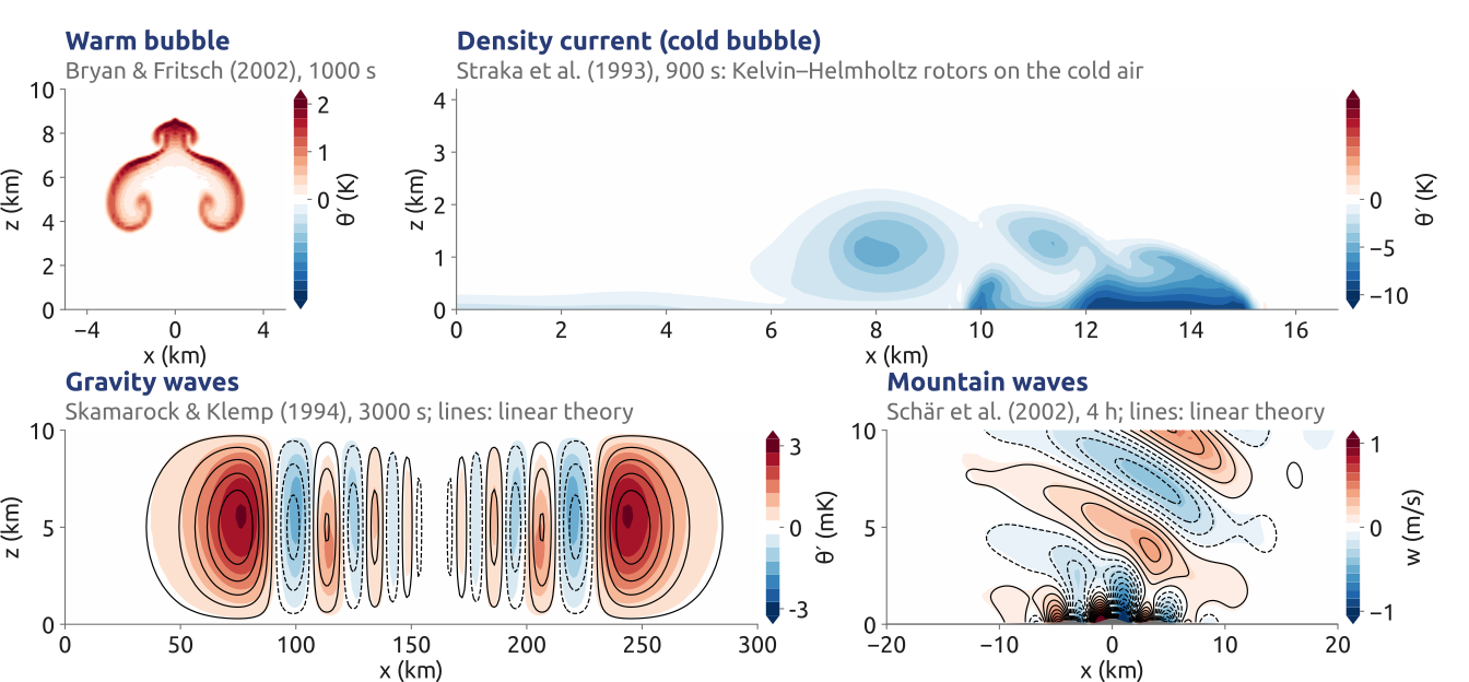
Shaded: Gusto runs of the compressible Euler equations; \(\theta'\): potential-temperature perturbation; \(w\): vertical velocity; lines: linear theory

Bubbles, density currents, gravity waves, mountains: the standard tests, here run with Gusto

(Bryan and Fritsch 2002; Straka et al. 1993; Skamarock and Klemp 1994; Schär et al. 2002)

Run with Gusto (lecture 8), compressible Euler, cells of 200 m to 1 km. Each test checks something: the bubble, nonlinear advection and buoyancy; Straka, a converged nonlinear reference; Skamarock-Klemp, linear waves against theory (lines: max 2.80 vs 2.73 mK); Schaer, terrain (0.90 vs 0.89 m/s).

A compressible core on Straka’s test

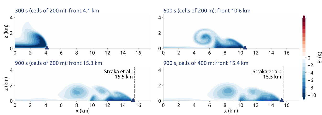
• Shaded: \(\theta'\), the potential-temperature perturbation; triangles: the front. Cells of 200 m: front at 15.3 km, 1.4% behind the reference (15.54 km); a Boussinesq slice model: 16.8 km, 8% ahead. The equations matter

• Gusto: velocity in \(H(\mathrm{div})\) (normal components continuous), \(\theta\) with \(w\) (Charney–Phillips); semi-implicit: one elliptic problem for the pressure per iteration

With the right equations and a converged reference, a model can be checked to the per cent

(Straka et al. 1993; Melvin et al. 2019; Natale et al. 2016)

Optional notebook 08e (lecture 8; Docker or Colab with Firedrake): where the unknowns sit, and Skamarock-Klemp against linear theory.

DCMIP: eleven cores, one set of tests

Model (centre)	Grid	Horizontal	Staggering	Vertical	Time
ACME-A (Sandia, Colorado)	cubed sphere	spectral elements	A	Lorenz, floating mass	KGU53 Runge–Kutta
CSU (Colorado State)	geodesic	finite volumes	Z	Lorenz, height	Adams–Bashforth 3
DYNAMICO (IPSL)	geodesic	finite volumes	C	Lorenz, floating mass	ARK(2,3,2) IMEX
FV3 (GFDL)	cubed sphere	finite volumes	D	co-located, floating mass	forward–backward, semi-implicit
FVM (ECMWF)	octahedral	finite volumes	A	co-located, height	semi-implicit
GEM (ECCC)	Yin–Yang	finite differences	C	Charney–Phillips, log pressure	semi-implicit
ICON (MPI-M, DWD)	icosahedral triangles	finite volumes	C	Lorenz, height	predictor–corrector
MPAS (NCAR)	Voronoi	finite volumes	C	Lorenz, height	split-explicit
NICAM (Japan)	geodesic	finite volumes	A	Lorenz, height	split-explicit
OLAM (Duke, Miami)	geodesic	finite volumes	C	Lorenz, height, cut cells	Adams–Bashforth 2
Tempest (UC Davis)	cubed sphere	spectral elements	A	Lorenz, height	ARS(2,3,2) IMEX

NCAR, June 2016: a two-week summer school. Tests: a moist baroclinic wave, a tropical cyclone, a splitting supercell on a small planet

Staggering: Arakawa’s A, C, D grids; Z: vorticity, divergence and mass at the same points. Floating mass: Lagrangian vertical layers. IMEX: implicit–explicit Runge–Kutta (ARK, ARS)

Very different formulations, judged on the same tests

(Ullrich et al. 2017; Jablonowski and Williamson 2006)

DCMIP: the Dynamical Core Model Intercomparison Project, workshops in 2008, 2012 and 2016 (Ullrich et al. 2017, Tables 2–5). The baroclinic-wave test of Jablonowski and Williamson (2006) is the classic one. LFRic and the IFS proper are not in the table (FVM is ECMWF’s finite-volume research core).

Four dynamical cores of today

	MPAS, MONAN	FV3	ICON	LFRic
Centre	NCAR; INPE (Brazil)	GFDL; NOAA’s GFS since 2019	DWD, MPI-M	Met Office
Equations	compressible, non-hydrostatic	compressible, non-hydrostatic	compressible, non-hydrostatic	compressible, non-hydrostatic
Grid	Voronoi hexagons	cubed sphere	icosahedral triangles	cubed sphere
Space	finite volumes, C grid (TRiSK)	finite volumes, D grid	finite volumes, C grid	mixed finite elements
Time	split-explicit	forward–backward, implicit vertical	predictor–corrector	iterated semi-implicit semi-Lagrangian
Vertical	height, Lorenz	floating Lagrangian layers	height, Lorenz	height, Charney–Phillips

TRiSK: the C-grid scheme of Thuburn, Ringler, Skamarock and Klemp; floating Lagrangian layers: levels that move with the flow and are remapped

The same equations, four discretizations: every method of this course is in a model of today

(Skamarock et al. 2012; Harris and Lin 2013; Zängl et al. 2014; Melvin et al. 2019; Adams et al. 2019; Ullrich et al. 2017)

Ask first: which of these models would you choose for a regional refinement over Italy, and why? (MPAS or ICON: variable resolution; FV3: stretching and nesting.) LFRic is named after Lewis Fry Richardson. The IFS stays spectral (octahedral grid, SISL).

Dynamical cores in the BRICS countries

Country	Model (centre)	Grid	Method
Brazil	MONAN (INPE), MPAS-based	Voronoi	finite volumes (TRiSK)
Brazil	BAM (CPTEC/INPE)	Gaussian	spectral, semi-implicit, Eulerian or SL
Russia	SL-AV (Hydrometcentre)	reduced lat–lon	finite differences, SISL
India	HGFM / BFS (IITM)	cubic octahedral	spectral, SISL
India	NCUM (NCMRWF; the Met Office’s UM)	lat–lon, C grid	finite differences, SISL
China	GRAPES / CMA-GFS (CMA)	lat–lon	finite differences, SISL
China	YHGSM (NUDT)	Gaussian	spectral, SISL
South Africa	UM (SAWS; Met Office)	lat–lon, C grid	finite differences, SISL

SISL: semi-implicit semi-Lagrangian; SL: semi-Lagrangian; lat–lon: latitude–longitude

Semi-implicit semi-Lagrangian steps (SISL) on many grids: the workhorse of operational centres

(Figueroa et al. 2016; Krishna et al. 2025; Tolstykh et al. 2017; Brown et al. 2012; Jiang et al. 2021; Skamarock et al. 2012); GRAPES/CMA-GFS: Pedro’s BRICS 2026 talk

Other BRICS members (Egypt, Ethiopia, Iran, UAE, Indonesia) run WRF, ARPEGE or JMA-NHM: users, not developers, of dynamical cores. Candidate to cut if time is short.

What a weather app shows: four global models

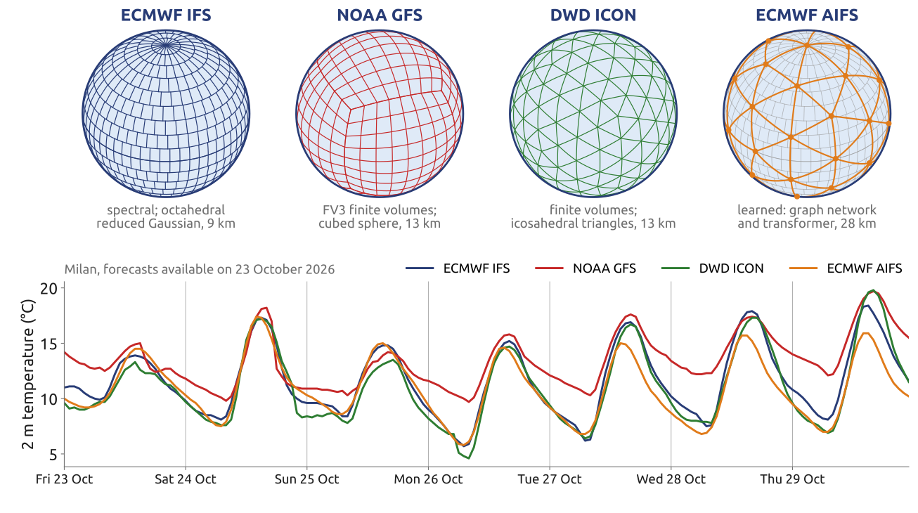
Windy.com shows the IFS, GFS, ICON and AIFS side by side: four grids, four methods, forecasts that differ by degrees

The forecast you read on your phone is one model among several, each with its own numerics

Data: open-meteo.com, forecasts available on 23 Oct. 2026 · App: windy.com

TODO (Pedro): Windy screenshots of the same forecast (model comparison), after checking the permission; the figure is ours: grids drawn coarse, temperatures from Open-Meteo for the same four models. Ask first: which model do you trust for Saturday? (The spread is the uncertainty: ensembles.)

Ocean models (1/3): the first one, 1969

\[\frac{D\mathbf u}{Dt} + f\,\mathbf k\times\mathbf u = -\frac{1}{\rho_0}\nabla\,\delta p + \mathbf F,\qquad \frac{\partial\,\delta p}{\partial z} = \rho_0 b,\qquad \nabla\cdot\mathbf u + \frac{\partial w}{\partial z} = 0\] \[\frac{DT}{Dt} = Q_T,\qquad \frac{DS}{Dt} = Q_S,\qquad b = b(T, S, z),\qquad {\color{#1f5ccc}w|_{z=0} = 0}\ \text{(rigid lid)}\]

\(\mathbf u = (u, v)\), \(w\): horizontal and vertical velocity; \(f\): Coriolis parameter; \(\rho_0\): reference density; \(\delta p\): pressure departure; \(b\): buoyancy; \(T\), \(S\): temperature, salinity; \(Q_T\), \(Q_S\), \(\mathbf F\): eddy mixing

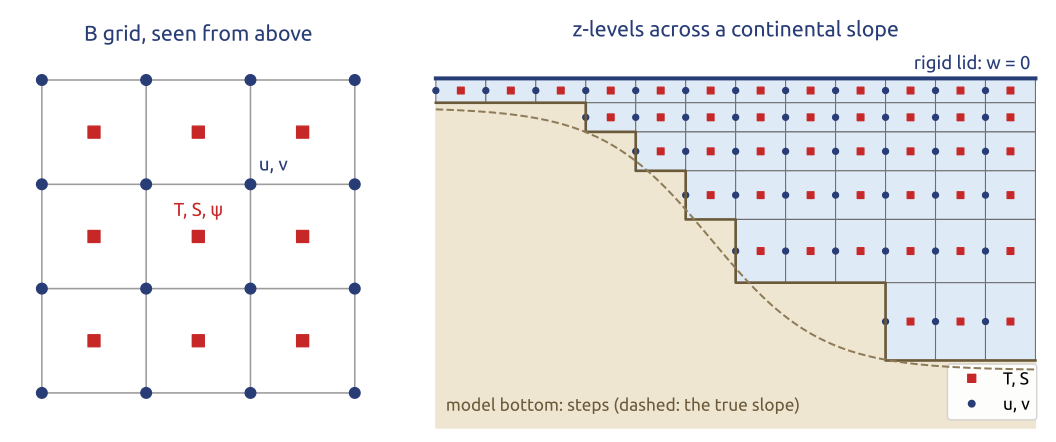
• Kirk Bryan, GFDL: the world ocean with coasts and bottom topography; z-levels, the B grid
• Rigid lid: no fast surface gravity waves (about 200 m/s); the depth-integrated flow from a streamfunction \(\psi\): an elliptic problem every step
• Manabe and Bryan (1969): the first coupled model; Bryan, Cox and Semtner’s code became GFDL’s MOM

1969: primitive equations on z-levels, a rigid lid, and an elliptic solve each step

(Bryan 1969; Manabe and Bryan 1969; Griffies et al. 2000)

Ask first: why a rigid lid? (Surface gravity waves at sqrt(gH), about 200 m/s, would force steps of minutes; the lid removes them. The price: an elliptic problem for psi, as in the 1950 forecast.) Bryan’s Fig. 2: T, S, psi at the centres, u, v at the corners (the B grid). Later models replaced the lid with a free surface.

Ocean models (2/3): the vertical coordinate

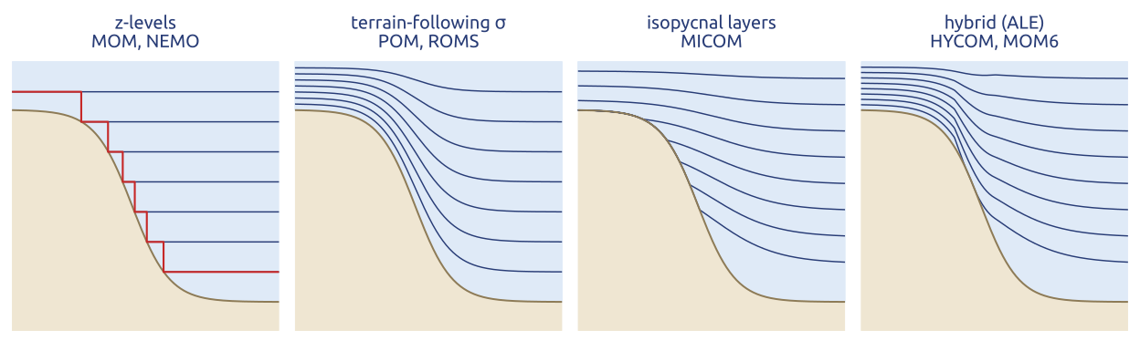
• z-levels (MOM, OPA/NEMO): simple, an exact horizontal pressure gradient; steps at the bottom, eased by partial steps
• Terrain-following \(\sigma\) (POM, ROMS): smooth over shelves and slopes, for coasts; the \(\sigma\) pressure-gradient error over steep slopes

• Isopycnal (MICOM): layers are density surfaces: no spurious mixing across them; they vanish where they outcrop
• Hybrid, ALE (arbitrary Lagrangian–Eulerian; HYCOM, MOM6): \(z\) near the surface, isopycnal inside, \(\sigma\) on the shelf
• A free surface replaces the rigid lid: a split-explicit barotropic mode (POM, ROMS)

Thirty years of debate on one choice: how the layers of the model follow the ocean

(Griffies et al. 2000; Blumberg and Mellor 1987; Shchepetkin and McWilliams 2005; Bleck 2002)

Ask first: why would an ocean model want its layers to be density surfaces? (The interior ocean mixes mostly along them; z-level advection adds spurious mixing across them.) The sigma error: the same as the atmosphere’s (sigma-coordinate slide). ALE: arbitrary Lagrangian–Eulerian. Bleck (2002): HYCOM, hybrid isopycnic-Cartesian.

Ocean models (3/3): the grids of today

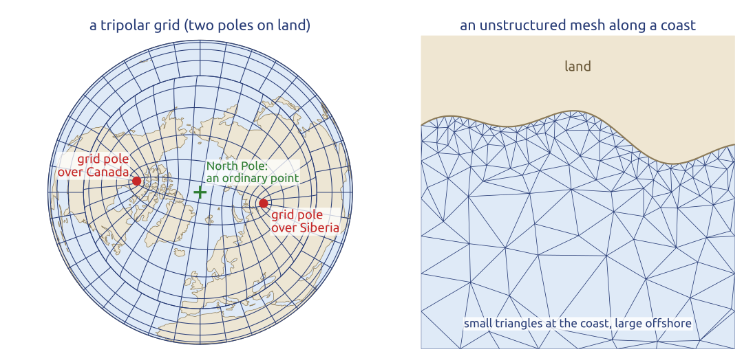
• The ocean’s pole problem is the North Pole, in the Arctic Ocean. Tripolar grids (Murray 1996) move the two northern grid poles onto land: NEMO’s ORCA grids, GFDL’s MOM
• MOM6 (Adcroft et al. 2019): C grid, a vertical Lagrangian-remap (ALE) coordinate, at \(1/4^\circ\) and \(1/2^\circ\)
• Unstructured meshes: FESOM2 (finite volumes), MPAS-Ocean (Voronoi), ICON-O (triangular C grid): small cells along coasts and straits, large ones elsewhere
• How fine? Gulf Stream simulations at \(1/8^\circ\) to \(1/64^\circ\) (Hurlburt and Hogan 2000)

Ocean grids moved their poles onto land, and their small cells to where the coasts are

(Murray 1996; Madec et al. 2026; Adcroft et al. 2019; Danilov et al. 2017; Ringler et al. 2013; Korn 2017; Hurlburt and Hogan 2000)

Ask first: why does the ocean have only one pole problem? (The South Pole is on land.) ORCA: NEMO’s tripolar family (ORCA1, ORCA025, ORCA12). Next slide: how fine an ocean grid must be, L_1 against the grid spacing.

The ocean’s eddies set the grid

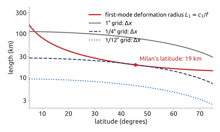
• Ocean eddies have the size of the first-mode deformation radius \(L_1 = c_1/f\) (\(c_1 \approx 2\) m/s: about 20 km at Milan’s latitude), against ~1000 km for the atmosphere’s cyclones
• At 45°N a \(1/4^\circ\) grid has about one cell per \(L_1\) (too coarse); a \(1/12^\circ\) grid has about three: \(L_1/\Delta x\) decides

\(c_1\): speed of the first baroclinic mode; \(f\): Coriolis parameter; \(\Delta x\): grid spacing

The ocean’s weather is ten times smaller: ocean models need ten times finer grids

(Vallis 2017; Cushman-Roisin and Beckers 2011)

L_1 and vertical coordinates: lecture 4 (c_1 = 2 m/s, L_1 about 20 km at Milan); L_d/dx: lecture 6. c_1 = 2 m/s at all latitudes (idealized; the real c_1 decreases poleward). L_d = NH/f of Vallis is π times larger. NEMO and MOM6: tripolar, finite volumes, Boussinesq and hydrostatic (lecture 3); FESOM2: unstructured triangles.

Key points

1. 1950 → the 1960s: from one equation to the primitive equations and general circulation models; Lorenz: chaos, hence ensembles
2. Finite differences on latitude–longitude grids: the polar cells set the time step; semi-implicit semi-Lagrangian steps
3. Spectral transforms: no pole problem, easy semi-implicit solves; but \(N^3\) transforms and global communication: the scalability problem
4. Quasi-uniform grids: cubed sphere, icosahedral, Voronoi; local finite volumes and elements
5. The vertical: Charney–Phillips staggering; an implicit vertical for sound; a sponge at the top; terrain-following coordinates and their pressure-gradient error
6. Tests: bubbles, density currents, mountains; DCMIP: very different cores, the same tests
7. Ocean: rigid lid to free surface; \(z\), \(\sigma\), isopycnal and ALE; tripolar and unstructured grids; eddies need \(1/10^\circ\)

Notebook 09a (open in Colab · download): exercise 1 comes back there.

Today’s models assemble the methods of this course, each in its own way

Reading: (Williamson 2007; Staniforth and Thuburn 2012; Ullrich et al. 2017; Griffies et al. 2000; Randall et al. 2019)

Next: data-driven forecasts (lecture 10), from the box before the model, data assimilation.

Backup slides

Slides kept for reference, not shown in class.

Still open in the field

• Dynamical cores that scale to the kilometre on new computers (GPUs), conserving what the equations conserve
• Learned models that keep mass and energy, forecast extremes and stay stable in a changing climate
• Physics and learning together: hybrids, learned data assimilation

Thank you! The problem is old; the tools are yours now

(Bauer et al. 2021; Vallis 2017; Cushman-Roisin and Beckers 2011)

Course evaluation form: TBA.