Data-driven weather forecasts: assimilation, reanalysis and AI models
Atmosphere and Ocean Dynamics, Lecture 10: notes
The forecast chain, from observations to the forecast, and the data-driven models. These notes discuss data assimilation and 4D-Var, an inverse problem with the model and its adjoint inside; reanalyses and ERA5; the data-driven models trained on ERA5, which learn one 6-hour step and forecast by composing it, and GraphCast’s graph network on an icosahedral multi-mesh; what they do well and what they miss (extremes, conservation); end-to-end and hybrid models; and a small AI emulator of the Lorenz-96 system.
1 From 1950 to today: the forecast chain
The first computer forecast, in 1950, integrated one equation (barotropic vorticity) for one layer of air over North America, on a grid of 736 km. A global forecast today solves the full equations for the whole atmosphere, coupled to models of the ocean, the land surface and the sea ice, on grids of about 10 km with about 100 levels, and repeats it about fifty times from slightly different initial states: an ensemble. The chain has five links (Figure 1): observations; data assimilation, which turns them into an initial state (Bjerknes’ “diagnosis”); the model, a dynamical core for the resolved motions plus parameterizations of the unresolved processes (radiation, clouds, turbulence, convection); and the forecast (Bjerknes’ “prognosis”) (Bjerknes 1904; Kalnay 2003, Ch. 1).
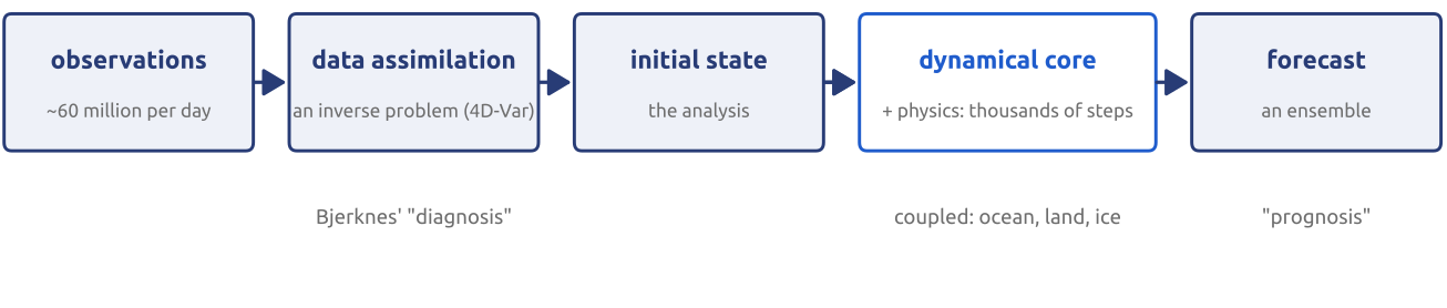
The skill of medium-range forecasts has grown by about one day per decade: a six-day forecast today is about as good as a five-day forecast ten years earlier (Bauer et al. 2015). The gains came from all the links at once: better models and higher resolution, far more observations (satellites), better data assimilation, and ensembles. Bauer, Thorpe and Brunet call it a “quiet revolution”: Bjerknes’ programme of 1904, observe, diagnose, integrate the laws, made industrial. Where does the initial state come from?
2 Observations: the global observing system
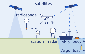
Every day ECMWF receives about 800 million observations, and about 60 million of them pass quality control and are available to its forecasting system (Modigliani et al. 2026) (Figure 2). Most come from about 90 satellite instruments. Satellites cannot measure temperature or humidity directly: microwave and infrared sounders measure radiances, from which temperature and humidity are inferred (spectroscopy); radio occultation infers them from the bending of GNSS signals through the atmosphere. Winds come from tracking clouds and water-vapour features and, near the ocean surface, from scatterometers; forecasts are still short of wind information. The in situ observations (surface stations, radiosondes, aircraft, ships, buoys, Argo floats) are few by comparison but direct and local: they calibrate and validate the satellite instruments, expose their biases and anchor the analysis. None of these is a model state: they are irregular in space and time, mostly indirect, and their errors differ from one instrument to the next.
3 Data assimilation: an inverse problem
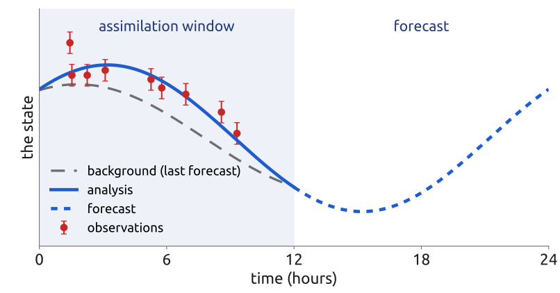
A forecast needs the state of the atmosphere at every grid point, about \(10^9\) numbers; what we have are the observations, irregular in space and time and mostly indirect: a satellite measures radiances, not winds or temperatures. Simply interpolating them onto the grid would leave most of the state undetermined and the rest unbalanced. Data assimilation finds instead the state most consistent with both the observations and a prior estimate, the background, which is the previous short-range forecast (Kalnay 2003, Ch. 5).
In four-dimensional variational assimilation (4D-Var) the analysis is the model trajectory over an assimilation window (6 to 12 hours) that best fits both the background and the observations of the window. The model is therefore inside the assimilation, and with it its adjoint; operational centres now combine it with ensembles of short forecasts to estimate the background errors (hybrid assimilation). The much improved analyses of the last decades account for a large part of the gain in forecast skill (Kalnay 2003, Sect. 5.6; Bauer et al. 2015). Figure 3 shows the idea on a toy problem with two unknowns.
4 4D-Var: a minimization problem
The unknown, or control variable, is the initial state \(x(t_0)\) of the window. 4D-Var minimizes \[ J[x(t_0)] = \tfrac12\,[x(t_0) - x^b]^{\mathsf T} \mathbf B_0^{-1} [x(t_0) - x^b] + \tfrac12\sum_{i=0}^{N} \bigl[H(x_i) - y^o_i\bigr]^{\mathsf T} \mathbf R_i^{-1} \bigl[H(x_i) - y^o_i\bigr], \qquad x_i = M(t_0, t_i)[x(t_0)], \] in the notation of Kalnay (2003, Sect. 5.6.3, eq. 5.6.14), where \(t_0, \dots, t_N\) are the observation times in the window (the index \(i\) counts only these times), \(x_i = x(t_i)\) the model state at \(t_i\), \(x^b\) the background, \(y^o_i\) the vector of all observations made at \(t_i\), \(H\) the observation operator, which maps a model state to what the instruments measure (radiances, for instance), \(M(t_0, t_i)\) the forecast model run from \(t_0\) to \(t_i\) (one model, run for longer for each later \(t_i\); Kalnay writes \(M_i\)), and \(\mathbf B_0\) and \(\mathbf R_i\) the error covariances of the background and of the observations. The first term, \(J_b\), keeps the analysis close to the last forecast where there are no observations: without it the problem is underdetermined, since there are far fewer observations than unknowns. The second, \(J_o\), pulls it towards the observations, each weighted by the inverse of its error covariance.
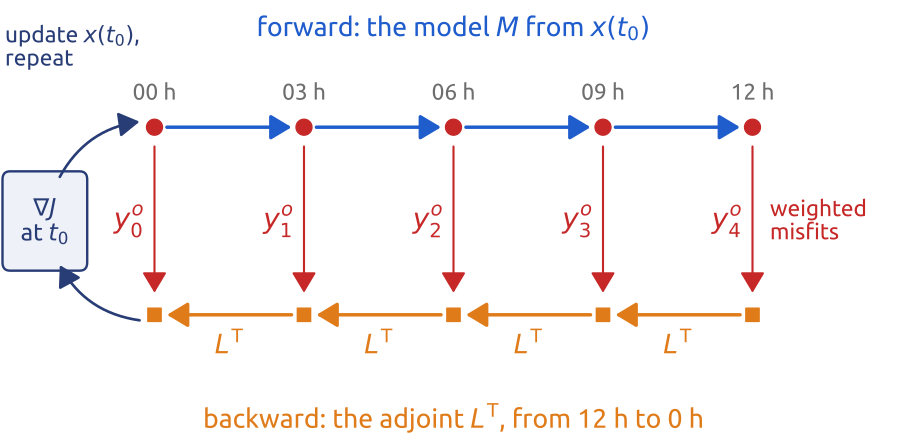
The minimization is iterative (conjugate gradient or quasi-Newton) and needs the gradient of \(J\) with respect to the \(10^9\) components of \(x(t_0)\). With \(\mathbf H_i\) the Jacobian of \(H\) at \(x_i\), \(L(t_0, t_i)\) the model linearized about the forward run (the tangent linear model), and \(L(t_i, t_0)^{\mathsf T}\) its adjoint, which carries a vector back from \(t_i\) to \(t_0\), Kalnay’s eqs. (5.6.17) and (5.6.19) give \[ \frac{\partial J}{\partial x(t_0)} = \mathbf B_0^{-1}[x(t_0) - x^b] + \sum_{i=0}^{N} L(t_i, t_0)^{\mathsf T}\, \mathbf H_i^{\mathsf T}\, \mathbf R_i^{-1} \bigl[H(x_i) - y^o_i\bigr]. \] Every iteration runs the model forward through the window, computes the weighted misfits \(\mathbf H_i^{\mathsf T}\mathbf R_i^{-1}[H(x_i) - y^o_i]\) at the observation times, and carries them back to \(t_0\) with the adjoint model \(L^{\mathsf T}\), which runs backwards in time and picks up each misfit on the way (Figure 4). The whole gradient costs a few model runs, whatever the number of unknowns. Because the analysis is a model trajectory (a strong constraint), it carries the model’s balances, and the forecast does not start with spurious gravity waves; the price is that the model is taken as perfect, and that \(\mathbf B_0\) must be known. In practice 4D-Var is incremental: the inner minimization uses a linearized model at lower resolution, and outer iterations update the trajectory at full resolution (Kalnay 2003, Sect. 5.6.3, pp. 181–184). A reanalysis needs decades of such analyses: with which model?
5 A reanalysis: decades of the past with one model
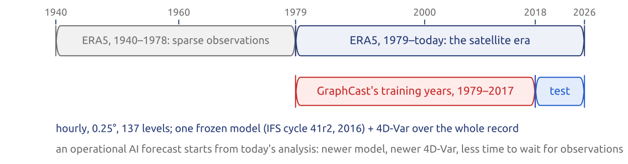
An analysis is the initial state of one forecast. The operational analyses of the past cannot simply be stacked into a record of the atmosphere: each was made with the model and the assimilation system of its day, and their improvements would look like climate change. A reanalysis repeats the analyses of the past, every day of decades, with one frozen model and one assimilation system. ERA5, produced by ECMWF for the Copernicus Climate Change Service, covers 1940 to today, hourly, at \(0.25^\circ\) (about 31 km) with 137 levels, about 5 PB of data; it was made with 4D-Var and the IFS of 2016 (cycle 41r2) (Hersbach et al. 2020) (Figure 5). Before the satellite era (1979) it rests on far fewer observations. It is the best estimate of the past atmosphere: one model and all the observations, together (Bauer et al. 2015).

ERA5 is free and openly licensed (CC BY 4.0), downloadable from the Copernicus Climate Data Store, on single levels (Copernicus Climate Change Service 2018b) and on pressure levels (Copernicus Climate Change Service 2018a), also from Python with the cdsapi package. This public good made data-driven forecasting possible.
6 ERA5 as training data
Four features of ERA5 matter for what a model learned from it can be (Figure 6). It is circular: made by the physics model that the learned models are meant to replace, a 2016 version of the IFS with 4D-Var, so “AI beats IFS” partly means “AI matches a 2016 IFS”. It is not homogeneous: the observations before the satellite era are far fewer, and the satellite constellation keeps growing. It is not available in real time: an ERA5 analysis uses observations from up to about 9 hours after its time, while an operational analysis must be ready after about 3 hours; a learned model is trained on one kind of initial state and run on another. And the training data is also the truth: the AI models are scored against ERA5, the IFS against its own analyses. GraphCast was trained on 1979–2017 and tested on 2018 and later (Lam et al. 2023; Hersbach et al. 2020). A learned model is only as good as the reanalysis it learns from, and that reanalysis is physics.
7 A new revolution: data-driven forecasts
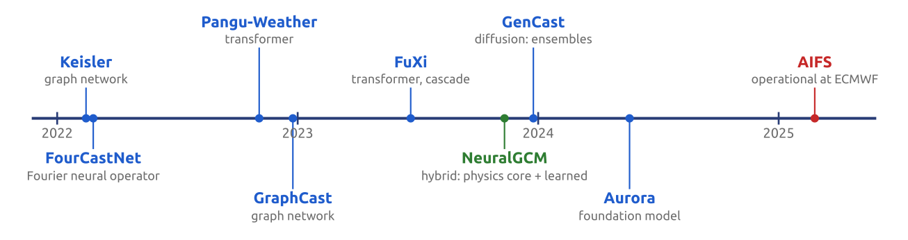
For a century, since Richardson, every forecast was computed by discretizing the equations of motion. Since 2022, models that learn the evolution of the atmosphere from data have matched, and on many scores beaten, the best physics-based global forecasts (Figure 7). In February 2022 Keisler showed a graph neural network forecasting at \(1^\circ\) (Keisler 2022) and NVIDIA released FourCastNet, a Fourier neural operator (Pathak et al. 2022); Huawei’s Pangu-Weather (Bi et al. 2023) and Google DeepMind’s GraphCast (Lam et al. 2023) appeared as preprints at the end of 2022 and in journals in 2023; FuXi followed (Chen et al. 2023). On 25 February 2025 ECMWF made its own data-driven model, AIFS, operational (Lang et al. 2024). In three years learned models went from a preprint to an operational forecast. What exactly do they learn?
8 Seven models in three years
The slide lists seven models, by the year of their first preprint, and what each brought:
| Year | Model | Who | What was new |
|---|---|---|---|
| 2022 | Keisler GNN (Keisler 2022) | Keisler | a graph neural network on a spherical mesh, encoder–processor–decoder; IFS-like skill at \(1^\circ\) |
| 2022 | FourCastNet (Pathak et al. 2022) | NVIDIA, LBNL, Caltech | Fourier neural operator; the first at the IFS’s own \(0.25^\circ\) |
| 2022 | Pangu-Weather (Bi et al. 2023) | Huawei | 3D transformer; the first to claim to beat the IFS deterministic forecast |
| 2022 | GraphCast (Lam et al. 2023) | Google DeepMind | a graph network on an icosahedral multi-mesh; better than the IFS on 90% of 1380 targets |
| 2023 | GenCast (Price et al. 2025) | Google DeepMind | diffusion: samples possible futures; better than the ECMWF ensemble on 97% of 1320 targets |
| 2023 | NeuralGCM (Kochkov et al. 2024) | Google, ECMWF, MIT | hybrid: a differentiable spectral core and learned physics |
| 2025 | AIFS (Lang et al. 2024) | ECMWF | graph transformer; the first operational data-driven model at a major centre (open) |
Each year brought a new kind of network: graph, Fourier operator, transformer, diffusion, hybrid. AIFS became operational on 25 February 2025 as a deterministic model; its ensemble followed later in 2025.
9 What is learned, and from what
A data-driven model learns a map \(\Phi_\theta\), with parameters \(\theta\), that advances the state by one step of 6 hours: \[ x^{n+1} = \Phi_\theta\!\left(x^{n}, x^{n-1}\right), \qquad \theta = \arg\min_\theta \sum_n \bigl\|\Phi_\theta(x^n, x^{n-1}) - x^{n+1}\bigr\|^2 , \] where \(x^n\) is the whole state at time \(n\), all the variables at all the points (for GraphCast, 227 variables, 5 at the surface and 6 on 37 pressure levels, at about \(10^6\) points: \(2.4\times10^8\) numbers), and the sum runs over the pairs of consecutive states of the training data (GraphCast uses the two previous states, as written here) (Lam et al. 2023). \(\Phi_\theta\) is not derived from the equations: it is fitted, a least-squares problem in millions of parameters. A 10-day forecast composes the step 40 times, where a physics-based model takes thousands of time steps. In practice the loss is weighted by latitude and by variable, and the training includes rollouts of several steps, so that errors do not grow too fast (Figure 8).
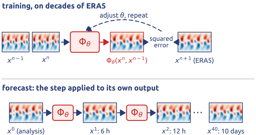
The training data is ERA5 (1940 to today, \(0.25^\circ\), 137 levels, hourly) (Hersbach et al. 2020), made by the physics model and 4D-Var. One box of the chain is replaced: the model is learned, but the initial state of every forecast still comes from physics.
10 Five families of learned models
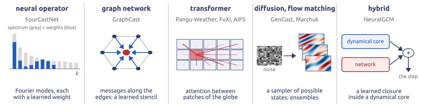
The networks differ; the task is the same, a map from the state now to the state 6 hours later (Figure 9):
- Neural operators (FourCastNet): each layer transforms the fields to Fourier space, multiplies the modes by learned weights and transforms back, a learned Fourier integral operator (Pathak et al. 2022).
- Graph networks (GraphCast): messages passed along the edges of a mesh, a learned stencil (Lam et al. 2023).
- Transformers (Pangu-Weather, FuXi, AIFS): attention between patches of the globe, each patch weighting all the others (Bi et al. 2023; Chen et al. 2023); AIFS has a graph-network encoder and decoder and a sliding-window transformer processor (Lang et al. 2024).
- Diffusion and flow matching (GenCast; Marchuk, AIRI, 2026): random noise turned step by step into possible states, an ensemble (Price et al. 2025).
- Hybrids (NeuralGCM): a discretized dynamical core with a learned closure for the unresolved processes (Kochkov et al. 2024).
What disappears in a learned model is the grid as an approximation of a continuous field, the CFL limit on the time step, and every conservation law; what survives is the state vector, and the initial state, which still comes from 4D-Var. The CFL condition disappears as a limit on the step, but not as a statement about domains of dependence (see the example below).
11 Inside a learned model: GraphCast
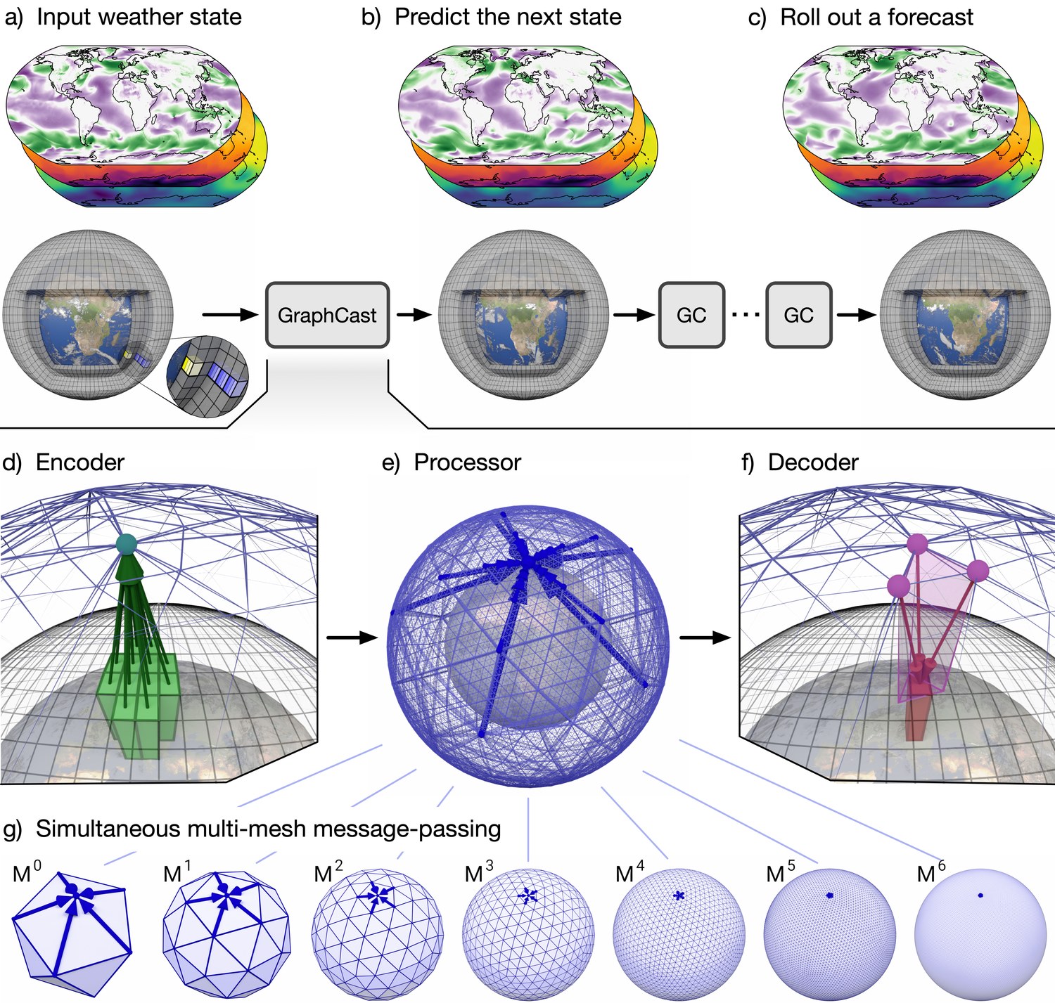
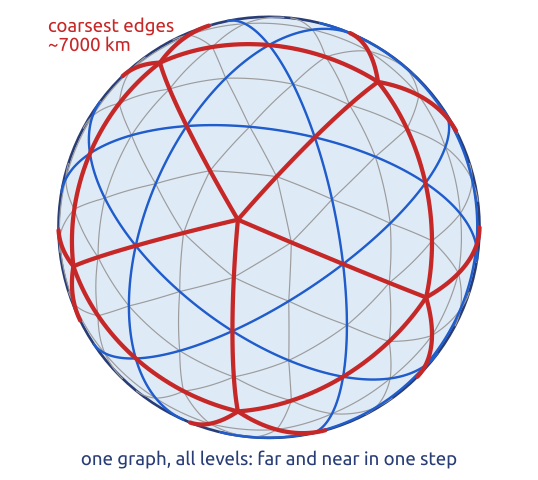
GraphCast (Lam et al. 2023) is an encoder–processor–decoder graph network, building on Keisler (2022) (Figure 10). (a–c) Its input is the state on the \(0.25^\circ\) grid, 227 variables (5 at the surface, 6 on 37 levels); it predicts the next state, and applied again and again it makes a forecast. (d) The encoder maps the grid onto a multi-mesh: the vertices of an icosahedron refined six times, 40 962 nodes. (e) The processor passes messages along the edges 16 times: each node updates its features from those of its neighbours, like a learned finite-volume flux, but repeated and nonlinear. (f) The decoder maps the result back to the grid, as the change of the state in 6 hours. (g) The multi-mesh keeps the edges of all seven meshes (the icosahedron and its six refinements) in one graph, from about 7000 km down to about 100 km: near and far at once (Figure 11).
The model has 36.7 million parameters; it was trained on ERA5 from 1979 to 2017, with rollouts of 1 to 12 steps, for about four weeks on 32 TPUs, and it makes a 10-day forecast in under a minute on one TPU, where the IFS takes about an hour on a supercomputer (Lam et al. 2023). Grids are back: a learned operator on an icosahedral mesh, as in finite volumes. But the CFL condition forbids explicit steps of 6 hours on a 28 km grid: how can it take them?
12 One box replaced
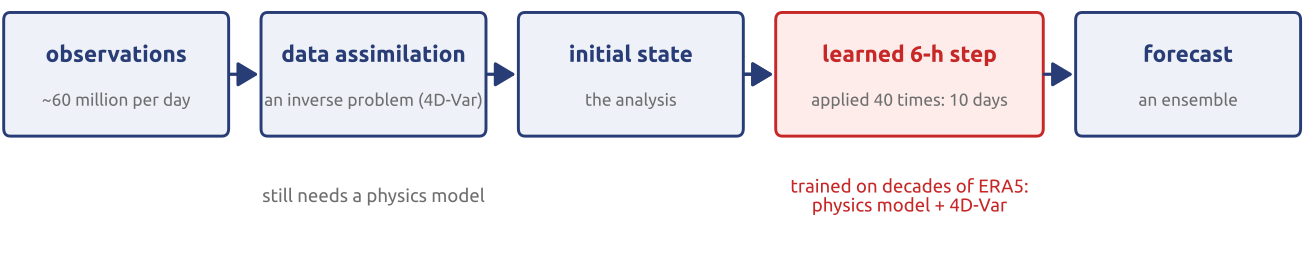
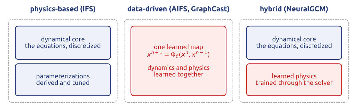
The chain of a data-driven forecast has the same links as that of a physics-based one, with the model box replaced by a learned 6-hour step, applied 40 times for a 10-day forecast, where the physics model takes about 1200 steps of 12 minutes (Figure 12). Four consequences:
- It still needs physics to run: the initial state comes from 4D-Var, and 4D-Var needs a model and its adjoint.
- Its training data needs a physics model: ERA5 is the IFS plus 4D-Var (Hersbach et al. 2020).
- Resolution is not the metric: AIFS, at 28 km, beats the IFS at 9 km on many scores (Lang et al. 2024).
- The physics–dynamics split is gone: dynamics and parameterizations are learned together; neither can be inspected or swapped, as a parameterization can in a physics-based model.
The learned step replaces the model; observations, assimilation and reanalysis remain (Bauer et al. 2015).
13 Example: how can an AI model take a 6-hour step?
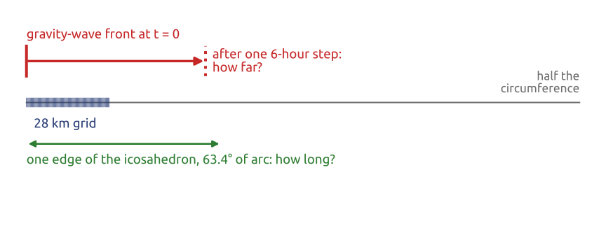
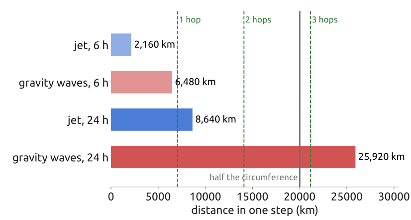
The example asks three questions (Figure 13):
- How far does a gravity wave travel in 6 hours at 300 m/s? How many explicit steps would a 28 km grid need for those 6 hours (CFL)?
- The learned model takes one step: how far apart are the two ends of an edge of the icosahedron (\(63.4^\circ\) of arc), the coarsest edges of GraphCast’s mesh?
- And for a step of 24 hours, with the jet stream (100 m/s) and the gravity waves?
14 What the example shows
Six hours. At 300 m/s a gravity wave travels \(300\ \text{m/s}\times 21\,600\ \text{s} = 6480\) km. On a 28 km grid the CFL condition with Courant number 1 allows explicit steps of at most \(28\ \text{km}/300\ \text{m/s} = 93\) s: about 230 steps for those 6 hours (Courant et al. 1928).
One edge. An edge of the icosahedron, \(63.4^\circ\) of arc on a sphere of radius 6371 km, is \(1.107 \times 6371 \approx 7050\) km long: longer than the domain of dependence of a 6-hour step. The multi-mesh keeps the 40 962 nodes of the finest mesh and the edges of all seven levels, about 7000, 3500, 1800, 900, 450, 220 and 110 km long; a node has the edges of the level at which it first appears and of the finer ones, so only the 12 vertices of the icosahedron carry the longest edges, as hubs (Lam et al. 2023). A typical node, with edges of about 110 km, reaches them in a few hops through coarser and coarser nodes (edges of 110, 220, 450, … km), crosses, and comes down: a few of the 16 rounds of message passing. The receptive field of one step covers the domain of dependence: the same idea as a semi-Lagrangian scheme, which puts the domain of dependence inside the stencil.
Twenty-four hours. The jet stream carries information \(100\ \text{m/s}\times 86\,400\ \text{s} = 8640\) km, about two hops of 7050 km; gravity waves travel 25 900 km, more than half the circumference (20 000 km). A 24-hour step needs a global receptive field; three hops of 7050 km reach anywhere, and GraphCast’s processor makes 16 (Figure 14). A learned step is a stencil: it must reach as far as the fastest signal travels in one step.
15 Do they work? Yes, mostly
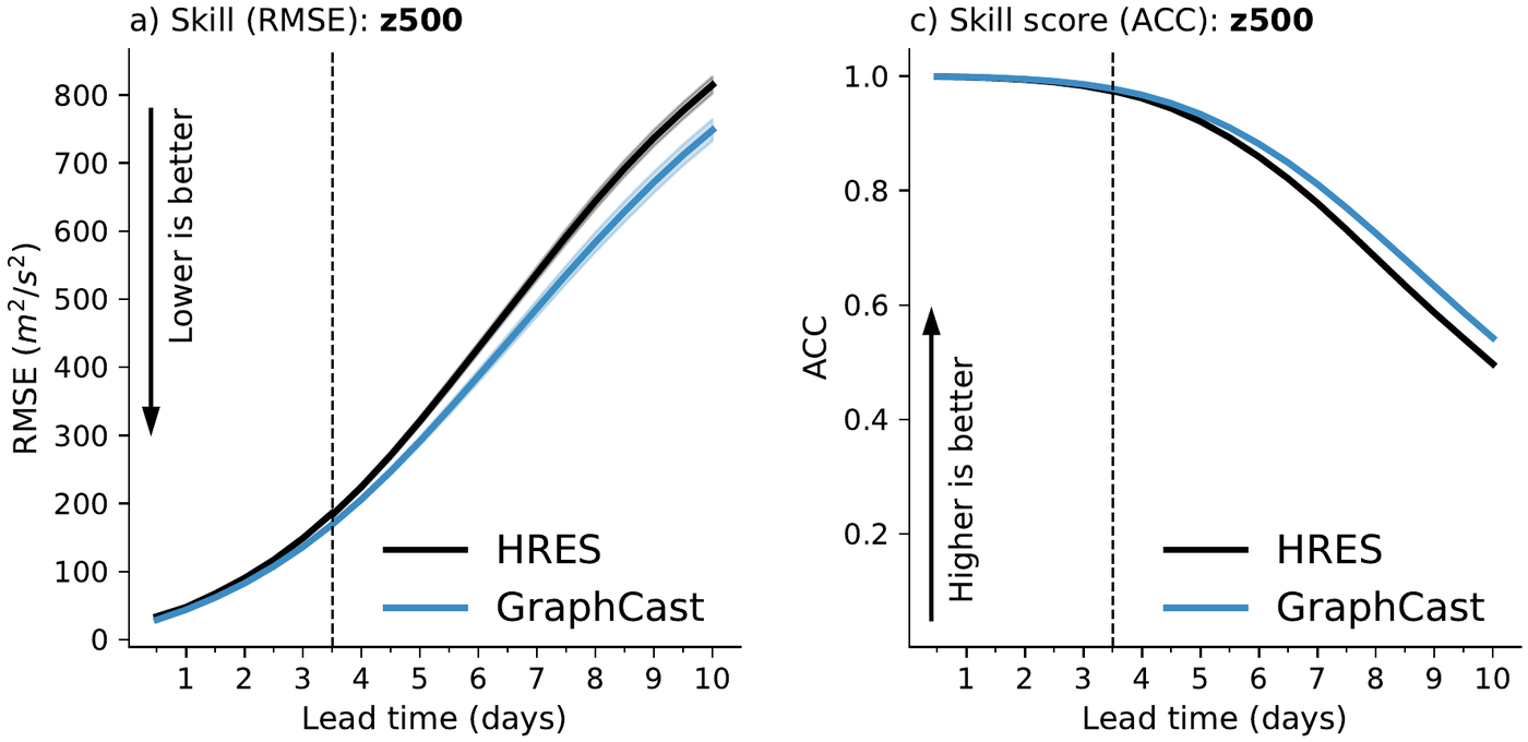
On the standard scores (root-mean-square errors and anomaly correlations of the main variables at many lead times), GraphCast beat ECMWF’s deterministic forecast, HRES, on 90% of 1380 targets (Lam et al. 2023) (Figure 15), and GenCast, a diffusion model, beat ECMWF’s ensemble on 97% of 1320 targets (Price et al. 2025). Open benchmarks such as WeatherBench 2 compare the models on the same footing (Rasp et al. 2024), and ECMWF has assessed them in an operational-like setting (Ben Bouallègue et al. 2024). AIFS, at 28 km, beats physics-based models at 9 km on many scores (Moldovan et al. 2026); once trained, it needs about a thousand times less energy per forecast than the physics-based model (ECMWF news, 25 February 2025). The scores carry a caveat: the AI models are scored against ERA5, the physics-based models against their own analyses.
What does not work, yet: the forecasts blur, because a model trained on the mean-square error forecasts the average of the possible futures; extremes are rare in the data; nothing enforces conservation laws; and the models need 4D-Var, a reanalysis and the climate of their training years. The next section takes these one by one.
16 What AI models cannot do, yet
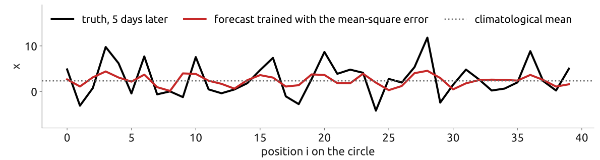
- Extremes. Record-breaking heat, cold and wind are forecast better by physics-based models (IFS-HRES) than by the AI models (Zhang et al. 2026): extremes are rare in the training data, and the mean-square error pulls the forecast towards the mean.
- Blurring. The forecast that minimizes the mean-square error is the mean of the possible futures, which is smooth: fronts and storm centres are smeared out as the lead time grows (Figure 16). Diffusion models such as GenCast sample sharp possible states instead of averaging them (Price et al. 2025).
- No conservation laws. Nothing in the network enforces the conservation of mass or energy; long runs drift. Hybrids keep a dynamical core for this reason, among others (Kochkov et al. 2024).
- Circular data. ERA5 is a physics product, and it is not available in real time.
- A changing climate. The models are trained on the past (GraphCast on 1979–2017) and used in the climate of today; they learn the climate of their training period.
17 The newest: learning the analysis too
Every model so far starts from a physics-based analysis: 4D-Var, the model trajectory that best fits the background and the observations (Figure 3). The newest systems learn this box too. End to end, they learn the map from the raw observations to the forecast, with no 4D-Var at run time. Aardvark Weather (Cambridge and the Alan Turing Institute) has an encoder from the observations to a gridded state, a processor and decoders to the forecasts (Allen et al. 2025); FuXi-Weather (Fudan) cycles data assimilation and forecast with learned models (Sun et al. 2025). Both are still trained on reanalyses, and still behind the best operational systems on many scores. The last box of the chain is being learned, from the observations straight to the forecast; without a physics model anywhere, who checks the learned atmosphere?
18 Where it is going: hybrids, and the world
Three ways to fill the model box are now in use (Figure 17). Hybrid models combine the two approaches: NeuralGCM keeps a differentiable spectral dynamical core and learns only the effect of the unresolved processes, training through the solver (Kochkov et al. 2024): the equations come back. Foundation models such as Aurora pretrain one large network on many data sets and fine-tune it to weather, air quality or ocean waves (Bodnar et al. 2025). And ensembles come from diffusion models, GenCast and FuXi-ENS, which sample possible futures instead of averaging them (Price et al. 2025; Zhong et al. 2025). The likely future is physics and learning together, not one replacing the other.
19 A tiny AI weather model
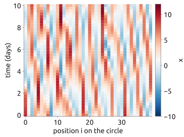
The whole idea fits on a laptop, in numpy, with the Lorenz-96 model as the “atmosphere” (Lorenz 1996): \(K = 40\) variables \(x_i\) on a latitude circle (periodic), \[ \frac{dx_i}{dt} = (x_{i+1} - x_{i-2})\,x_{i-1} - x_i + F , \] with \(F = 8\), chaotic (Figure 18). The quadratic term is an advection, \(-x_i\) a damping and \(F\) a forcing; Lorenz chose the time unit so that 0.05 is about 6 hours of the atmosphere. The computation takes the steps in turn: the model, integrated with RK4 and steps of 0.01, after a spin-up that drops the transient from rest; a “reanalysis”, a long run of 16 000 states 6 hours apart (about 11 “years”) for training and a separate run for testing; the 6-hour step learned by least squares, first as a linear map \(x^{n+1} = x^n + Wx^n + \mathbf b\) (1640 parameters, seeing the whole circle), then by a small network with a local stencil, \(x_{i-2}, \dots, x_{i+2}\), two hidden layers of 32 and the same weights at every point (1281 parameters); forecasts by composing the step 40 times; and a model fitted to the mean-square error 5 days ahead, which blurs. Which forecasts better, the linear model or the small network?
20 What the notebook showed
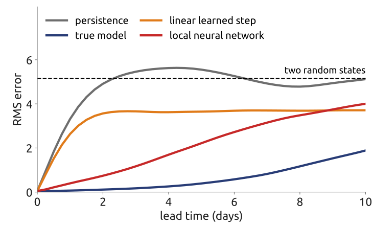
The one-step errors are 0.78 for the linear model and 0.10 for the local network (RMS; the spread of the states is 3.6). From 200 test states with initial errors of 0.05, the RMS errors at days 1 and 5 are 3.3 and 5.6 for persistence, 2.6 and 3.7 for the linear model, 0.40 and 2.2 for the local network, and 0.07 and 0.39 for the true model started from the same wrong state (Figure 19). The local network, with fewer parameters, beats the linear model: it was given the right structure, a local rule that is the same everywhere, like a finite-difference stencil, and its sensitivities to \(x_{i-2}, \dots, x_{i+2}\) equal those of the true 6-hour step. Its stencil must cover where information comes from in one step: a stencil of width 3, which misses \(x_{i-2}\), fails (RMS error 2 at day 1), width 5 works: the CFL condition, learned. The linear model decays to the mean: its error stops at about the spread of the states. Nothing beats the true model from a slightly wrong start for long: its error is the initial error amplified by chaos, and the network’s one-step error costs it about five days of predictability. A learned step is a numerical method whose coefficients were fitted instead of derived.
21 Key points
- The initial state: data assimilation, an inverse problem with the model inside (4D-Var).
- Reanalysis: decades of analyses with one frozen model; ERA5 is what AI models learn from.
- Learned models: a 6-hour step fitted to ERA5; it must see as far as the fastest signal goes: CFL, learned.
- One box replaced: the observations, the assimilation and the reanalysis remain physics.
- Do they work? Excellent average forecasts; extremes, conservation and a changing climate remain open.
- The newest: learning the analysis too (end to end); hybrids keep the equations.
AI replaces one box of the chain: the observations and the physics around it remain.
22 The course in one chain
| Topic | What you can now do |
|---|---|
| History | tell the story from Halley to the 1950 forecast, and why rotation matters |
| Laws | derive the equations, reduce them to shallow water, find their waves and balances |
| Vertical | treat the vertical: buoyancy, internal waves, convection, mountain waves |
| Grids | discretize them with finite differences and volumes; stability, CFL, conservation |
| Spectral, FE | spectral methods and finite elements: the cores of IFS and LFRic |
| Models | follow the models from 1950 to today: grids, the vertical, the tests |
| AI | read the chain of a modern forecast and what learned models change in it |
Bjerknes’ two conditions of 1904, a sufficiently accurate knowledge of the state of the atmosphere at an initial time and of the laws by which one state develops from another, organize the whole course (Bjerknes 1904): the laws, their reduction and their discretization, and the initial state and the forecast chain (Bauer et al. 2015). What remains open is as much mathematics as engineering: dynamical cores that scale to the kilometre on new computers; learned models that conserve what the equations conserve, forecast extremes and stay reliable in a changing climate; and the coupling of both. The problem is old; the tools are yours now.
Further reading
Bauer et al. (2015) on the progress of numerical weather prediction; Kalnay (2003), Chapter 5, on data assimilation and 4D-Var; Hersbach et al. (2020) on ERA5; Lam et al. (2023) and Price et al. (2025) for two learned models in detail, Rasp et al. (2024) for how they are compared, and Zhang et al. (2026) for their extremes.